Week 3 - Solving second order ODEs

PROGRAM THAT SOLVES THE ODE REPRESENTING EQUATION OF MOTION OF SIMPLE PENDULUM WITH DAMPING

Above equation is a second order ordinary differential equation representing following terms:

(b)damping coefficient= 0.05

(l) length of pendulum in meters= 1m

(g) gravity=9.81 m/s^2

(m) mass of ball in kg= 1 kg

angular velocity (v)=3 rad/sec

angular displacement is given 0 in the problem and

time limit is given between 0 to 20 sec.

FOLLOWING IS THE PROGRAM WRITTEN FOR SOLVING SECOND ORDER ODE:

Here in the program, ode45 is used and it is a solver in matlab which is used to calculate angular velocity and angular displacement for the given time span.

%SOLVING SECOND ORDER DIFFERENTIAL EQUATION USING MATLAB

clear all
close all
clc
 
%FOLLOWING ARE THE INPUTS
b = 0.05; % b is damping coefficient
T = 1; % mass
g = 9.81; % gravity
l = 1; % length


% INPUTS CONDITIONS
theta_0= [0 ; 3] ; % where angular diplacement is taken as 0 and angular velocity is taken as 3 rad/sec

% TIME INPUT
t_span= linspace(0,20,550);  % time limit is given in the problem is 0 to 20 seconds

% SOLVING THE ODE
[t, results]= ode45(@(t,theta) ode_funct(t, theta, b,g,l,T),t_span,theta_0);

% plotting
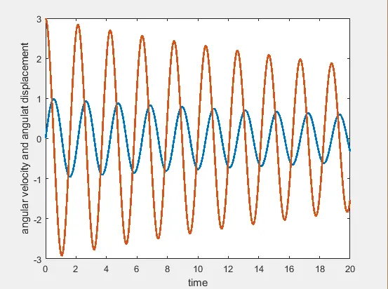
plot(t,results(:,1),'linewidth',2);
hold on
plot(t, results(:,2),'linewidth',2);
xlabel('time');
ylabel('angular velocity and angulat displacement');

RESULTS OBTAINED FROM THE ABOVE PROGRAM IS SHOWN BELOW:

So in the other program second order differential equation converted into first order by calling the function in the above written program and program for function that is used in the above program is written below:

function [dtheta_dt]=ode_funct(t,theta,b,g,l,m) %calling a function

theta1=theta(1);
theta2=theta(2);

dtheta1_dt=theta2;
dtheta2_dt= -(b/m)*theta2-(g/l)*sin(theta1);

dtheta_dt=[dtheta1_dt;dtheta2_dt];
end

Now, moving to the pendulum animation:

Program for the pendulum animation is written below:

Here 'for' command is used to create the loop for the pendulum animation and lengths are fixed in the 3rd and the 4th coordinates using (x0,y0) and (x1,y1) as shown in the below program.

Also, Marker command is used to create a graphical object and 'spherical object' is created using marker command.

theta=results(:,1);



% PENDULUM ANIMATION
ct=1;

for i= 1:length(theta)
    angle=theta(i);
    figure(2)
    title('simple pendulum')
    x0=0;
    y0=0;
    
    x1=l*cos(3*pi/2+angle);
    y1=l*sin(3*pi/2+angle);
    
    plot([x0,x1],[y0,y1],'linewidth',2)
    hold on
    plot(x1,y1,'o','markers',20)
    hold on
    plot([-3,3],[0,0],'linewidth',3)
    hold off
    axis([-5,5,-2,2])
    pause(0.02)
    M(ct)=getframe(gcf);
    ct=ct+1;
end
    
% MAKING THE ANIMATION FILE
movie(M)
videofile=VideoWriter('simplependulum.avi','Uncompressed AVI');
open(videofile)
writeVideo(videofile,M)
close(videofile)    

following is the pendulum, animation obtained from the above programming:

https://youtu.be/NUOWyHktv-s