Week 4.1 - Genetic Algorithm
Theroy and introductions
the generatic algorithm is inspried by the process that drives biological evaliation. the process of evaluation starts with the selsction fittest individals from the population. they the produce offspring which inherrit the characteristic of the parents and will be added to the next generation. if parents have better have better fitness their offspring will be batter than parents and the have a better generation.
the fittest individuls will be founds and uses them to produce the childen forth next geeratio. over succesive genneration, the population evolves towards an optimal solution. the generitic algorithm that are not well suitable for standerd optization algorith, i which the objects function is discontinus, nondifferentiable, stachastic or higher nonlinear.
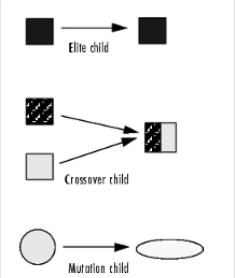
The genetic algorithm uses three main types of rules at each step to create the next generation from the current population.
. selected the rules selected the individual, called parents that contribute to the population at the next generation.
. crossover rules combine two parents to from children for the next generation.
. muntation rules apply random change to individul parents to from children.
Algorithm working sequence
algorithm then creates a sequecce of new population. at each the algorithm uses the individual in the current generation to create the next population. to create the new population it uses fitness function which is the function you want to optimize . for standered optimization algorithm this is known as the objective function. the toolbox softare tries to find the minimum of the fitness function.
The algorithm performs the following steps
. The algorithm begines by create a random a random initialpopulation.
. then it scale the raw fitness score to convert them into a more usable range of values thes scaled valus are called expenction values.
. then it selected members called parents based based on their expectations.
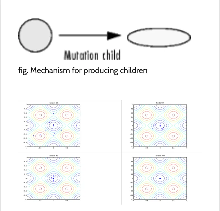
. it them repalce the current the current population with the chidren to from the next generation.
. then it score each member of the current population by computing ti's fitness values these values are called the raw fitness score.
. them the algorithm when one of the stopping criteria is met.
inputs function:-
f(x,y) = f1,xf2,xf3,yf2,y
f1.x = [sin(5.1pi.x+0.5)]^6
f1,y = [sin(5.1pi.y+0.5)]^6
f2,x = exp[-4ln(2)(x-0.0667)^2/0.64]
f2,y = exp[-4ln(2)(y-0.0667)^2/0.64]
the stalagmite function to plot the graph in the main functions.
function (f) = stalagmite(input_value)
f1x = (sin(5.1*pi*input_value(1) +0.5)).^6;
f1y = (sin(5.1*pi*input_value(2) + 0.5)).^6;
f2x = exp(-log(2)*(((input_value(1) - 0.0667).^2/0.64)));
f2y = exp(-4*log(2)*(((input_value(2) - 0.0667).^2/(0.64)));
f = -(f1x*f1y*f2x*f2y);
end
main body
the mesh from the two vector which will be acting as a serach space to find the maxima of the function.
creating the mesh of this two vectors using the mesh command and definig the number of iteration as nun_cases to iteration the vlue of the optimum value of the function.
now calculate the values of fitnes function at each point of the mesh grid formed.
now creating the value of fitness function at each of the mesh grid formed.
now creating its surface throuugh 'surfc' command which will also provides the contour of the generated surface.
MATLAB CODE:
clear all
close all
clc
x = linspace(0,0.6,150);
y = linspace(0,0.6,150);
num_cases = 50;
% creating a 2D mesh
[xx,yy] = meshgrid(x,y);
%evaluating stalagmite function
for i = 1:lenght(xx)
for = 1:length(yy)
inputs_value(1)=xx(i,j);
input_value(2)=yy(i,j);
f(i,j) = stalagmite(input_value);
end
end
% study1-unbounded statistical behaviourtic
for i = 1:nun_cases
[inputs1,fopt2(i)] = ga(@stalagmite, 2);
xopt(i) = inputs1(1);
yopt(i) = inputs1(2);
end
study1_time = toc;
figure(1)
subplot(2,1,1)
hold on
surfc(xx,yy,-f)
xlabel('x-values')
y label(y-values')
zlabel('function values')
shading interp
plots(xopt,-fopt,'marker','o','markersize',5,'markerfacecolor','r')
title('unbounded statistical behaviour')
subplot(2,1,2)
plot(-fopt1)
xlabel('iterations')
ylabel('function maximum')
% study2 - statistical behaviour with upper and lower bound
tic
for i = 1:num_cases
[inputs2,fopt2(i)] = ga(@stalagmite,2,[],[],[],[]
xopt(i) = inputs2(1);
yopt(i) = inputs2(2);
end
study2_time = toc
figure(2)
subplot(2,1,1)
hold on
surfc(xx,yy,-f)
xlabel('x-values')
ylabel('y-values')
zlabel('function values')
shading interp
olot3(xopt,yopt,-fopt,'marker','o','markersize',5,'markerfacecolor','r')
title('bounded statisticalbehaviour')
subplot(2,1,2)
plot(-fopt2)
xlabel('iterations')
ylabel('function maximum')
% study3- increasing GA iterations ( populationsize)
options = optimoptions('ga');
option = optimoptions(options,'populationsize',170);
tic
for i= 1num_cases
[inputs3, fopt3(i)] = ga(@stalagmite,2,[],[],[][],[0,0],[1:1],[],[],options)
xopt(i) = inputs3(1);
yopt(i) = inputs3(2);
end
study3_time = toc
figure (3)
subplot(2,1,1)
hold on
surfc (xx,yy,-f)
xlabel('x-values')
ylabel9'y-values")
zlabel('function values')
shading interp
plot(xopt,yopt,-fopt,'marker'','o','markersize',5,'markerfacecolor','r')
title('bounded statistical popluation size')
subplot(2,1,2)
plot(-fopt3)
xlabel('iterations;)
ylabel('function maximum')
fprintf('n the results are below :')
fprintf('nn stduy 1: unbounded statistical bahaviour')
fprintf('nn the time for the study-1 is : %f' , study1_time) fprintf('n the co-ordinates of x & y for the global maxima of the function are ; %f, %f',inputs1(1),inputs1(2)) fprintf(' nn the global maxima of the function is : %f', -(mean(fopt)))
fprintf('nn study 2 : unbounded statistical bahaviour')
fprintf(' nn the time taken for t study-2 is : %f' ,study2_time)
fprintf('n the co-ordinate of x & y for the golbal maxima of of the function are : %f, %f',inputs2(1), inputs2(2))
fprintf('nn the global maxima of the function is :%f', -(mean(fopt2)))
fprintf('nn study 3 : unbounded statistical bahaviour')
fprintf('nn the time takn for the study-3 is : %f',study3_time)
fprintf('n the co-ordinate of x7y for the global maxima of the function is : %f', -(mean(fopt3)))
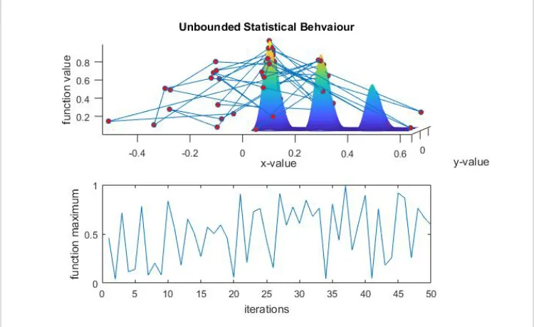
outputs 1.
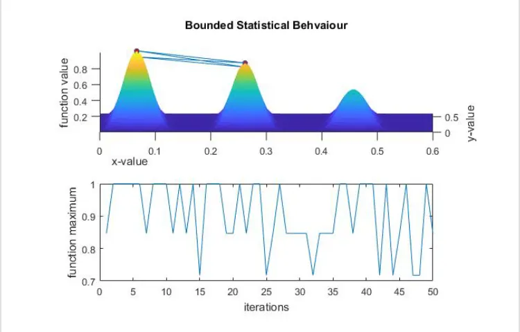
output 2.
outpu 3.
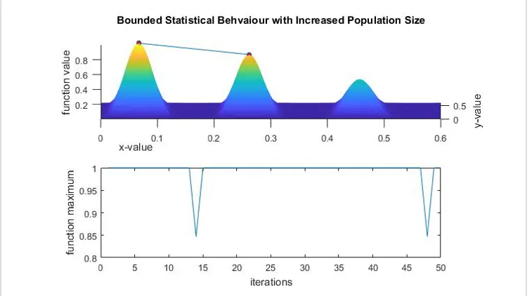
stalagmita function output print in command window
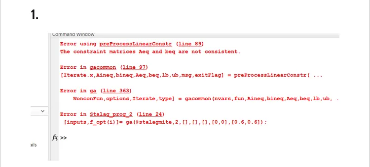
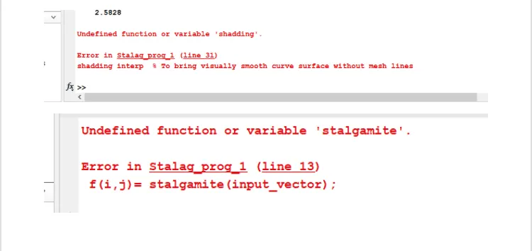
Error while programming:-
1.
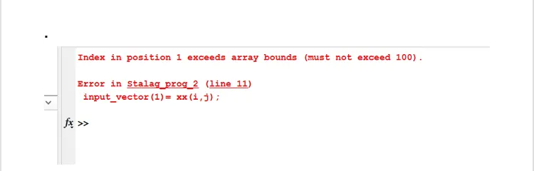
2.
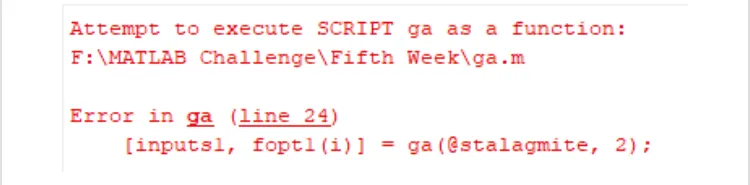
3.
1. unbounded ststistical behaviour-
the time taken for the study-1 = 5.912489
the global maxima of the function = 0.512086
2. unbounded ststistical behaviuor-
the time taken for the study-2 = 7.937613 sec
the global maxima of the function = 0.905461
3. bounded ststistical behaviour with increase populsion size-
the time taken for the study-3 = 19.544688 sec
the global maxima of the function = 0.993887
The total time taken to complete the total study 33.305790