Week 4.1 - Genetic Algorithm
Aim :- Write a code in MATLAB to optimise the stalagmite function and find the global maxima of the function.
Genetic Alogrithm :-
-
The genetic algorithm is a method for solving both constrained and unconstrained optimization problems that is based on natural selection the process that drives biological evolution.
-
The genetic algorithm repeatedly modifies a population of individual solutions. At each step the genetic algorithm selects individuals at random from the current population to be parents and uses them to produce the children for the next generation.
-
Over successive generations, the population 'evolves' toward an optimal solution.
-
We can apply the genetic algorithm to solve a variety of optimization problems that are not well suited for standard optimization algorithms including problems in which the objective function is discontinuous, non-differentiable, stochastic, or highly nonlinear.
-
The genetic algorithm can address problems of mixed integer programming where some components are restricted to be integer-valued.
The genetic algorithm uses three main types of rules at each step to create the next generation from the current population:
- Selection rules select the individuals, called parents that contribute to the population at the next generation.
- Crossover rules combine two parents to form children for the next generation.
- Mutation rules apply random changes to individual parents to form children.
The following line summarizes how to create the genetic algorithm works
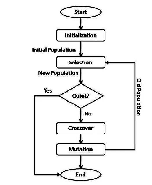
- The algorithm begins by creating a random initial population.
- The algorithm then creates a sequence of new populations. At each step, the algorithm uses the individuals in the current generation to create the next population. To create the new population, the algorithm performs the following steps
- Scores each member of the current population by computing its fitness value.These values are called the raw fitness scores.
- Scales the raw fitness scores to convert them into a more usable range of values.These scaled values are called expectation values.
- Selected members called parents based on their expectation.
- Some of the individuals in the current population that have lower fitness are chosen as These elite individuals are passed to the next population.
- Produces children from the parents.Children are produced either by making random changes to a single parent mutation or by combining the vector entries of a pair of parents crossover.
- Replaces the current population with the children to form the next generation.
3. The algorithm stops when one of the stopping criteria is met.
The flow chart for GA is given below,
The Stalagmite Function is used in these program is given below
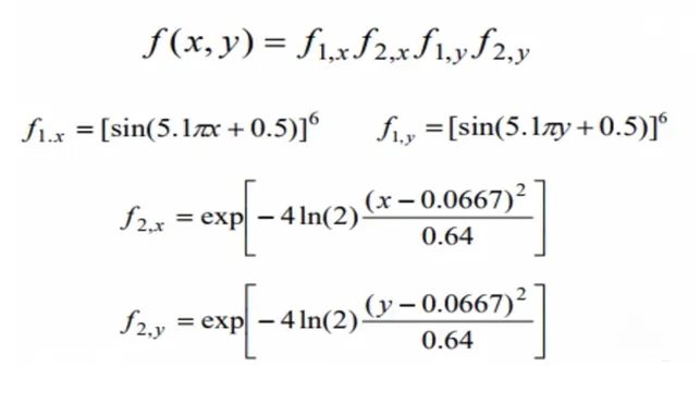
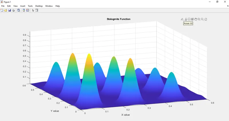
The above equations are used in the stalagmite function to plot the graph in the main functions.
There are three cases which we are going to study for following function.
a) Statistical Behaviour without boundation.
b) Statistical Behaviour with upper & lower boundation.
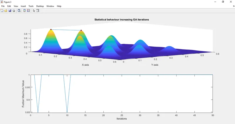
c) Statistical Behaviour with increaseing in GA iteration.
Syntax & Description :-
1) x = ga(fun,nvars), is uesd to finds a local unconstrained minimum 'x', to the objective function 'fun' , 'nvars' is the dimension (number of design variables) of fun.
2) x = ga(fun,nvars,A,b), is used to finds a local minimum x to fun, subject to the linear inequalities A*x ≤ b. 'ga' evaluates the matrix product A*x as if x is transposed (A*x').
3) x = ga(fun,nvars,A,b,Aeq,beq), finds a local minimum x to fun, subject to the linear equalities Aeq*x = beq & A*x ≤ b. (Set A=[] & b=[] if no linear inequalities exist) 'ga' evaluates the matrix product Aeq*x as if x is transposed(Aeq*x').
4) x = ga(fun,nvars,A,b,Aeq,beq,lb,ub), defines a set of lower and upper bounds on the design variables 'x', so that a solution is found in the range lb ≤ x ≤ ub. (Set Aeq=[] & beq=[] if no linear equalities exist).
5) x = ga(fun,nvars,A,b,Aeq,beq,lb,ub,nonlcon), subjects the minimization to the constraints defined in nonlcon. The function nonlcon accepts x and returns vectors c & Ceq, representing the nonlinear inequalities and equalities respectively. 'ga' minimizes the fun such that C(x) ≤ 0 and Ceq(x) = 0. (Set lb=[] & ub=[] if no bounds exist).
6) x = ga(fun,nvars,A,b,Aeq,beq,lb,ub,nonlcon,options), minimizes with the default optimization parameters replaced by values in options.(Set nonlcon=[] if no nonlinear constraints exist). Create options using optmoptions.
7) x = ga(fun,nvars,A,b,Aeq,beq,lb,ub,nonlcon,intcon) or x = ga(fun,nvars,A,b,Aeq,beq,lb,ub,nonlcon,intcon,options), requires that the variables listed in intcon take integer values.
8) x = ga(problem), finds the minimum for problem, a structure described in problem.
9) [x,fval] = ga(___), for any previous input arguments, also returns fval, the value of the fitness function at x.
10) [x,fval,exitflag,output] = ga(___), also returns exitflag, an integer identifying the reason the algorithm terminated, and output, a structure that contains output from each generation and other information about the performance of the algorithm.
11) [x,fval,exitflag,output,population,scores] = ga(___), also returns a matrix population, whose rows are the final population, and a vector scores, the scores of the final population.
Matlab Program :-
- Function Program :-
function[f] = stalagmite(input_vector)
x = input_vector(1);
y = input_vector(2);

t1 = (sin(5.1*pi*x + 0.5))^6;
t2 = (sin(5.1*pi*y + 0.5))^6;
t3 = exp(-4*log(2)*(x-0.0667)^2/0.64);
t4 = exp(-4*log(2)*(y-0.0667)^2/0.64);

f = -(t1*t2*t3*t4);
end
- Main Program :-
% Program to optimise the stalagmite function and find the global maxima of the function.
clear all
close all
clc

% Defining search space for function
x = linspace(0,0.6,150);
y = linspace(0,0.6,150);

% Creating a 2-Dimensional Mesh
[xx,yy] = meshgrid(x,y);

% No. of itreation for which the function will evaluate the fitness.
num_cases = 50;

% Creating the surface plot of Stalagamite Function
for i = 1:length(xx)
    for j = 1:length(yy)
        input_vector(1) = xx(i,j);
        input_vector(2) = yy(i,j);
        f(i,j) = stalagmite(input_vector);
    end
end
% Generating the surface
surfc(xx,yy,-f)
xlabel('x value')
ylabel('y value')
shading interp
[inputs,fval] = ga(@stalagmite,2);

% Study 1 - Statistical behaviour without boundation.
tic
for i = 1:num_cases
    [inputs,fopt(i)] = ga(@stalagmite,2);
    xopt(i) = inputs(1);
    yopt(i) = inputs(2);
end
study1_time = toc
figure(1)
subplot(2,1,1)
hold on
surfc(xx,yy,-f)
shading interp
xlabel('X-axis')
ylabel('Y-axis')
plot3(xopt,yopt,-fopt,'marker','o','markersize',5,'markerfacecolor','r')
title('Statistical behaviour without boundation')
subplot(2,1,2)
plot(-fopt)
xlabel('Iterations')
ylabel('Fuction Maximum Value')

% Study 2 - Statistical behaviour with upper & lower boundation.
tic
for i = 1:num_cases
    [inputs,fopt(i)] = ga(@stalagmite,2,[],[],[],[],[0;0],[1;1]);
    xopt(i) = inputs(1);
    yopt(i) = inputs(2);
end
study2_time = toc
figure(2)
subplot(2,1,1)
hold on
surfc(xx,yy,-f)
shading interp
xlabel('X-axis')
ylabel('Y-axis')
plot3(xopt,yopt,-fopt,'marker','o','markersize',5,'markerfacecolor','r')
title('Statistical behaviour with upper & lower boundation')
subplot(2,1,2)
plot(-fopt)
xlabel('Iterations')
ylabel('Fuction Maximum Value')

% Study 3 - Statistical behaviour increasing GA iterations.
tic
options = optimoptions('ga');
options = optimoptions(options,'PopulationSize',170);
for i = 1:num_cases
    [inputs,fopt(i)] = ga(@stalagmite,2,[],[],[],[],[0;0],[1;1],[],[],options);
    xopt(i) = inputs(1);
    yopt(i) = inputs(2);
end
study3_time = toc
figure(3)
subplot(2,1,1)
hold on
surfc(xx,yy,-f)
shading interp
xlabel('X-axis')
ylabel('Y-axis')
plot3(xopt,yopt,-fopt,'marker','o','markersize',5,'markerfacecolor','r')
title('Statistical behaviour increasing GA iterations')
subplot(2,1,2)
plot(-fopt)
xlabel('Iterations')
ylabel('Fuction Maximum Value')

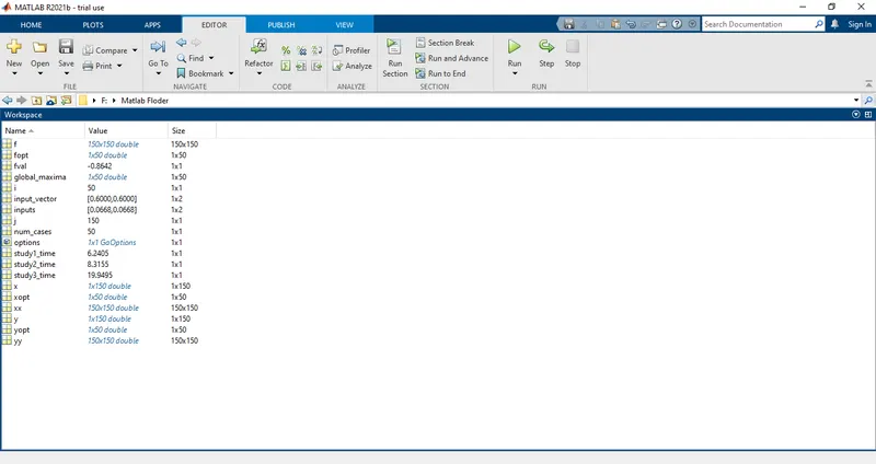
global_maxima = -fopt
Explation :-
- First we will creating the mesh from the two vectors which will acting as a search space to find the maxima of the function.
- Then 'Mesh' command is used to create the mesh of these two vectors.
- Now, calculating the values of fitness function at each point of the mesh grid formed.
- Now, defining the no. of iterations as num_cases to iterate the values of the function.
- Using the 'for loop' to creating the surface plot of stalagmite function.
- Now, by 'surfc' command we will create its surface.
- While using surfc applying '-ve' sign to the function will generate the surface upside down which will be use to get the maxima of the function.
- Now, we will study three cases which are mention above program.
1) Case Study 1 :- Statistical Behaviour without boundation.
a) In this evaluating the optimum value of fitness of function at each iteration & calculating it using the above mentioned syntax in the intro part, which gives the input i.e. value of x & y at which the stalagmite functionis minimum but for maximum we are using '-ve' sign.
b) Then plotting it into the 'surfc' command & also providing the optimum values of the function that how it is varying.
c) Also using the 'tic & toc' command to evalute the time used for optimizing the function.
2) Case Study 2 :- Statistical Behaviour with upper & lower boundation.
a) The difference over here is that, by providing upper & lower limits in the ga so that the search space is reduced with upper & lower boundary.
b) And then plotting it as similar to the above study.
3) Case Study 3 :- Statistical Behaviour by increasing GA iterations.
a) In this study, using 'optimoptions' command to increase the size of population.
b) The benefit of these is, it will be working on the large set of nos. & which will be led to increase the possibilities of finding the better fitness of the function.
c) The drawback of these, the time for evalution will increase.
Plots & Graphs :-
1) The 3-D surface generated for randam sampling
2) The plot & graph for case study 1
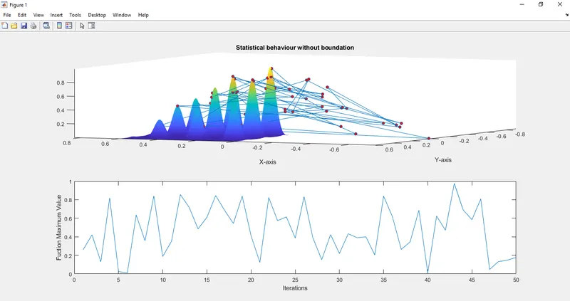
From the above figure, it is clear that the results are not that much accurate and giving a lot of variation in optimizing the function.
3) The plot & graph for case study 2
From the above figure, it is clearly seen that after providing the boundary limits the variation in the optimum value of the function has reduced.
4) The plot & graph for case study 3
5) Workspace
6) Global Maxima

References :-