Week 3 - Solving second order ODEs
Aim :- Write a program to solve the second ODE of motion of a pendulum with damping & and create an animation file.
- Second ODE of motion of a pendulum with damping.
- Create an animation file for it.
A simple example is pendulum.The way the pendulum moves depends on the Netwon second law of motion.When this law is written down we get a second order Ordinary Differential Equation that describes the position of the ball with respect to time.This ODE represents the equation of motion of a simple pendulum with damping.The equation is given below
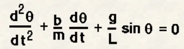
where,
g = gravity in m/s2.
L = length of the pendulum in m.
m = mass of the ball in kg.
b = damping coefficient.
For above expression,
L = 1 meter, m = 1 kg, b = 0.05, g = 9.81 m/s2.
Time interval = 0-20 sec, for angular displacement = 0, & angular velocity = 3 rad/sec at time = 0.
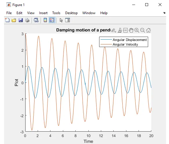
First we will define the inputs & variables i.e., damping coefficient, gravity, length of pendulum, mass of ball.After that we will define the initial condition i.e., angular displacement, angular velocity with time span.Then to solve ODE, we use ode45 which is inbuild command in Matlab to solve the ODE using a numerical method while using this command we have to use the function program to be integrated to calculated the time span & the inital condition w.r.t time.After these calculation the graph is to plotted, the graph is contain the two plots i.e one is angular displacement & one is angular velocity w.r.t time.
Now for loop is used, before we add a counter loop, for loop allows us to write a loop that need to execute a specific number of times,the starting & ending points are defined. The loop is used for all the values of time span are assigned to a varabile 'i' one at a time.The values for x0,x1,y0 & y1 are given. Then plotting command is used to plot the view of a simple pendulum, title command is used to give the title to the plot, axis command is used to fixexd the axis where the pendulum is oscillated.After that pause command is used to get proper view of position where pendulum is oscillating.By getframe command we will get every frame & store in varaible 'M'.Then increment for loop execauted, movie commands is used to create the movie for output of graph which is obtain by running these program & to save in the hard drive. And in last the you tube link is shared.
Matlab code :-
 % Write a program to solve the second ODE of motion of a pendulum with damping & and create an animation file.

 % Inputs
 b = 0.05;   % Damping coefficient.
 g = 9.81;   % Gravity in m/s^2.
 l = 1;      % Lenght of pendulum in m.
 m = 1;      % Mass of ball in kg.

 % Inital Condition
 theta_0 = [0;3];  % Angular displacement & Angular velocity in rad/sec

 % Time Points between 0 to 20 sec
 t_span = linspace(0,20,500);

 % Solve ODE
 [t,results] = ode45(@(t,theta) ode_func(t,theta,b,g,l,m),t_span,theta_0);

 % Plotting
 figure(1)
 hold on
 plot(t,results(:,1))
 plot(t,results(:,2))
 title('Damping motion of a pendulum')
 legend('Angular Displacement','Angular Velocity')
 xlabel('Time')
 ylabel('Plot')

 % For Loop
 ct = 1;
 for i = 1: length(results(:,1))
     x0 = 0;
     y0 = 0;
     x1 = l*sin(results(i,1));
     y1 = -l*cos(results(i,1));

     % Plotting the animation
     figure(2)
     plot([-1 1],[0,0],'linewidth',4)
     hold on
     plot([x0 x1],[y0 y1],'linewidth',4)
     hold on

     plot(x1,y1,'o','markersize',20,'MarkerFaceColor','b')
     title('Animation of a simple pendulum')
     axis([-1.5 1.5 -1.5 0.1])
     grid on
     pause(0.003)
     hold off
     M(ct)=getframe(gcf);
     ct =ct+1;
 end
 % Animation movie of a simple pendulum
 movie(M)
 videofile=VideoWriter('Pendulum Animation.avi');
 open(videofile)
 writeVideo(videofile,M)
 close(videofile)
Function Program :-
function [dtheta_dt] = ode_func(t,theta,b,g,l,m)

   theta1 = theta(1)
   theta2 = theta(2)
   dtheta1_dt = theta2;
   dtheta2_dt = -(b/m)*theta2 - (g/l)*sin(theta1);
   dtheta_dt = [dtheta1_dt ; dtheta2_dt];
end
Output :-
You tube link :-