Week 4.1 - Genetic Algorithm

Aim:

To write MATLAB code to optimize Stalagmite function and to find the global maxima of the function.

Theory:

The genetic algorithm 'GA' is a method for solving both constrained and unconstrained optimisation problems that is based on natural selection; a process that drives biological evolution.

GA repeatedly modifies the population of individual solutions.

At each step, the genetic algorith selects individuals at random from the current population to be parents and uses them to produce children for the next generation.

Over successive generations, the population evolves towards an optimal solution.

GA can be applied to solve a variety of optimization problems that are not suitable for standard algorithms, including problems in which the function is discontinuous, non differential, stochastic, or highly non linear.

the GA uses 3 main types of rules at each step to create the next generation from current population:

1. Selection rule selects the individuals, called parents, that contribute to the population at the next generation.
2. Crossover rule combines two parents to form children for the next generation.
3. Mutation rule applies random changes to individual parents to form children.

Procedure:

Overview:

1. First, Stalagmite Function is defined in a separate script.
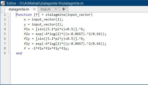
2. A negative sign is used in function to obtain maxima of the function rather than the minima.
3. A nested 'for loop' is utilized to iterate each of the elements i.e. a 2D array for results of Stalagmite function is created.
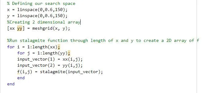
4. GA is used to determine the optimal of the function.
5. Plot is generated for differnt cases:
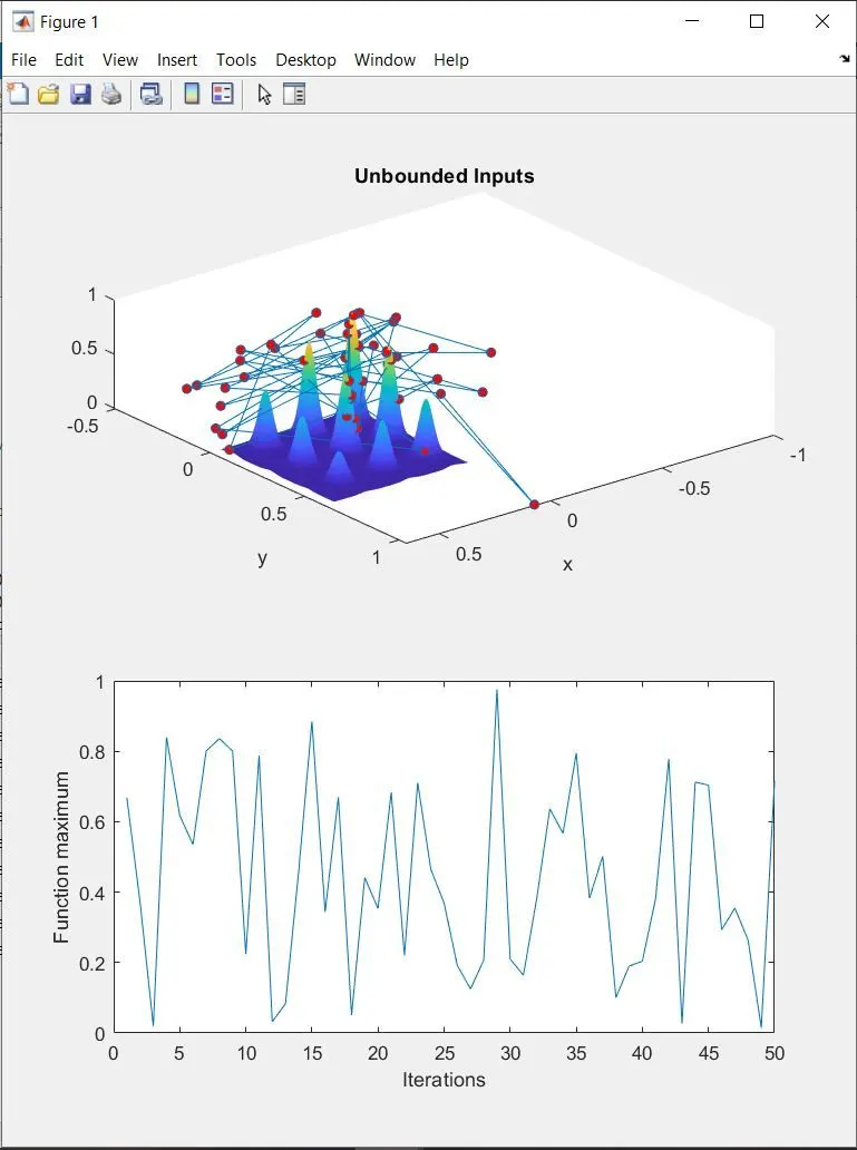
   1. Unbounded Inputs : Syntax used: x = ga(fun,nvars) finds a local unconstrained minimum, x, to the objective function, fun. nvars is the dimension (number of design variables) of fun.
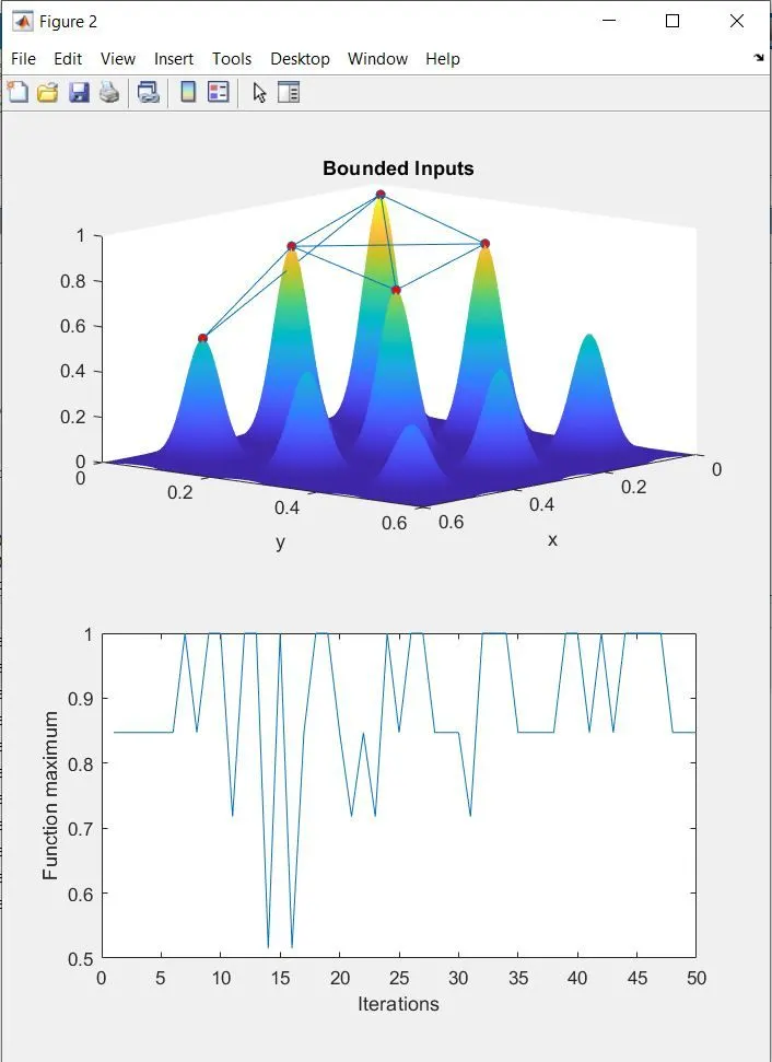
   2. Bounded Inputs: Syntax used: x = ga(fun,nvars,A,b,Aeq,beq,lb,ub) defines a set of lower and upper bounds on the design variables, x, so that a solution is found in the range lb ≤ x ≤ ub. (Set Aeq=[] and beq=[] if no linear equalities exist.)
   3. Bounded Inputes with defining(increasing) the population size: Syntax used: x = ga(fun,nvars,A,b,Aeq,beq,lb,ub,nonlcon,options) minimizes with the default optimization parameters replaced by values in options. (Set nonlcon=[] if no nonlinear constraints exist.) Create options using optimoptions.

MATLAB Code:

clear all
close all
clc
% Defining our search space
x = linspace(0,0.6,150);
y = linspace(0,0.6,150);
%Creating 2 dimensional array
[xx yy] = meshgrid(x, y);

%Run stalagmite function through length of x and y to create a 2D array of f
for i = 1:length(xx);
    for j = 1:length(yy);
    input_vector(1) = xx(i,j);
    input_vector(2) = yy(i,j);
    f(i,j) = stalagmite(input_vector);
    end
end

%-------------------------------------------------
tic
% Run genetic algorithm 50 times(iterations)
% recording calculated value of ga for 50 iterations in fopt and it's
% position in xopt and y opt
rep = 50;
for i = 1:rep
    [Inputs2, fopt(i)] = ga(@stalagmite, 2);
    xopt(i) = Inputs2(1);
    yopt(i) = Inputs2(2);
end
Study_time = toc

figure(1)
subplot(2,1,1);
hold on
surf(xx,yy,-f)
shading interp
plot3(xopt, yopt, -fopt, 'marker', 'o', 'MarkerSize',5,'MarkerFaceColor','r')
title('Unbounded Inputs')
xlabel('x')
ylabel('y')
subplot(2,1,2)
plot(-fopt)
xlabel('Iterations')
ylabel('Function maximum')

%------------------------------------------------------

tic
% Run genetic algorithm 50 times(iterations)
% recording calculated value of ga for 50 iterations in fopt and it's
% position in xopt and y opt
%
% study2 - Statistical behaviour under upper bound and lower bound
for i = 1:rep
    [Inputs2, fopt(i)] = ga(@stalagmite, 2, [],[],[],[],[0;0],[1;1]);
    xopt(i) = Inputs2(1);
    yopt(i) = Inputs2(2);
end
Study_time2 = toc

figure(2)
subplot(2,1,1);
hold on
surf(xx,yy,-f)
shading interp
plot3(xopt, yopt, -fopt, 'marker', 'o', 'MarkerSize',5,'MarkerFaceColor','r')
title('Bounded Inputs')
xlabel('x')
ylabel('y')
subplot(2,1,2)
plot(-fopt)
xlabel('Iterations')
ylabel('Function maximum')

%------------------------------------------------------

tic
% Run genetic algorithm 50 times(iterations)
% recording calculated value of ga for 50 iterations in fopt and it's
% position in xopt and y opt
%
% study3 - Statistical behaviour under upper bound and lower bound and
% mentioning the population size
% By default, Population size is 50, which maybe small for our problem and
% will lead to output of a local maxima; increasing population size will
% give us a global macima as output

options = optimoptions('ga')
options = optimoptions(options, 'Populationsize', 170);

for i = 1:rep
    [Inputs2, fopt(i)] = ga(@stalagmite, 2, [],[],[],[],[0;0],[1;1],[],[],options);
    xopt(i) = Inputs2(1);
    yopt(i) = Inputs2(2);
end
Study_time3 = toc

figure(3)
subplot(2,1,1);
hold on
surf(xx,yy,-f)
shading interp
plot3(xopt, yopt, -fopt, 'marker', 'o', 'MarkerSize',5,'MarkerFaceColor','r')
title('Bounded Inputs')
xlabel('x')
ylabel('y')
subplot(2,1,2)
plot(-fopt)
xlabel('Iterations')
ylabel('Function maximum')

Results:

Case 1: Unbounded Inputs

Case 2: Bounded Inputs; defined Upper bound and Lower bound.

Case 3:Bounded Inputs with increased population size.

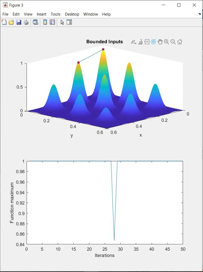
Conclusion:

Case 3 gives us a optimum result, as the upper bound and lower bound are defined as well as the Population size has been increased to 170, which will provide a global result by virtue of increased number of iterations.