Project 2 - Rankine cycle Simulator

Aim :

To simulate the Rankine cycle and plot the TS HS Plots using MATLAB

Objective :

1. Calculate the state points of Rankine cycle based on given inputs.
2. Plot the corresponding TS HS plots.

Input Values:

1. Turbine Inlet temperature = 400 C
2. Turbine Inlet pressure = 30 bars
3. Turbine Outlet Pressure = 0.05 bars

Required Outputs:

1. Net work output
2. Back work ratio
3. Plots for TS and HS

Theory:

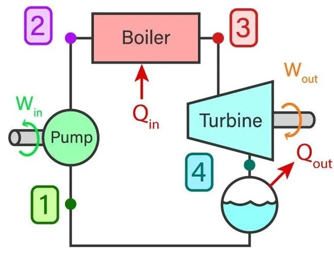
Above is the Process diagram for Rankine cycle.

1. Rankine cycle is an ideal cycle for comparing the performance of steam plants. It is modified form of Carnot cycle, in which the condesation process is continued until the steam is condensed into water.
2. Rankine cycle uses Steam as a working substance.
3. The cycle is completed by following 4 processes:
   1. Process 1-2: The saturated water at point 1 is isothermally converted into dry saturated steam in a boiler, and the heat is absorbed at a constant temperature T1 and pressure P1. The dry state of steam is represented by point 2. It means that T2 and P2 is equal to temperature T1 and P1 respectively.
   2. Process 2-3: The dry saturated steam at point 2, now expands isentropically in an engine or turbine. The pressure and temperature falls from p2 to p3 and T2 to T3 respectively with a dryness fraction x3. SInce no heat is supplied or rejected during the process, therefore there is no change of entropy.
   3. Process 3-4: The wet steam at point 3 is now isothermally condensed in a condenser and the heat is rejected at constant temperature T3 and pressure P3 untill the whole steam is condensed into water. It means that the temperature T4 and pressure P4 is equal to the temperature T3 and pressure P3 respectively.
   4. Process 4-1: The water at point 4 is now warmed in a boiler at constant volume from temperaure T4 to T1. Its pressure also rises from P4 to P1. The heat absorbed by water during the process p1, i.e. equal to sensible heat at point 1 minus sensible heat at point 4.

Code format:

1. All required parameters, variables and inputs are found out.
2. Using the 'XSteam' library, values for all parameters required for calculation are obtained.
3. Obtained variables are put into formulas to get the required output.
4. Plotting for graphs are done as per the theory of thermodynamics.

Code explaination:

1. input function is used to get required inputs.

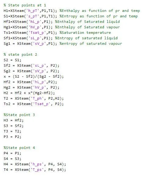
2. Using the XSteam library the values such as Hf, Hg, Ts, Sf, Sg are obtained. 'XSteam' function from thhe XSteam library is used; Syntax for XSteam function is XSteam('function name [for example, h_pT is code name for enthalpy as a function of pressure and temperature], Input1 i.e. pressure, Input2 i.e. temperature)

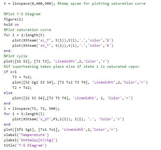
3.Use linspace command to create temperature space for plotting saturation curve.

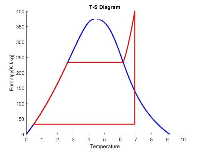
For plotting T-S diagram, first plot the saturation curve and then plot the cycle. For plotting cycle, use if else as there are 2 options, 1 being if steam reaches superheated state other being if steam on reached saturated steam state.

Give X label, Y label and Heading to the plot.

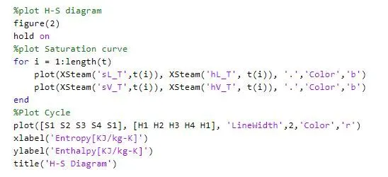
4. Plot H-S diagram.

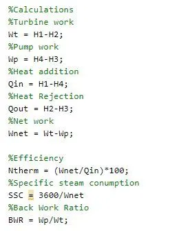
5. Calculate the required outputs and store inrespective variables.

6. Use fprintf command to print the output in the command window.

Syntax for fprintf command: fprintf('string for output', previously stored variable as output answer)

Code:

clear all
close all
clc

P1 = input('\nEnter the pressure at turbine inlet (in bars):\n');
P2 = input('\nEnter the pressure at turbine outlet (in bars):\n');
T1 = input('Enter the temperature at turbine inlet (in Degree Celcius):\n');


% State points at 1
H1=XSteam('h_pT',P1,T1); %Enthalpy as function of pr and temp
S1=XSteam('s_pT',P1,T1); %Entropy as function of pr and temp
Hf1=XSteam('hL_p',P1); %Enthalpy of Saturated liquid 
Hg1=XSteam('hV_p',P1); %Enthalpy of Saturated vapour
Ts1=XSteam('Tsat_p',P1); %Saturation temperature
Sf1=XSteam('sL_p',P1); %Entropy of saturated liquid
Sg1 = XSteam('sV_p',P1); %entropy of saturated vapour

% state point 2
S2 = S1;
Sf2 = XSteam('sL_p', P2);
Sg2 = XSteam('sV_p', P2);
x = (S2 - Sf2)/(Sg2 - Sf2);
Hf2 = XSteam('hL_p',P2);
Hg2 = XSteam('hV_p', P2);
H2 = Hf2 + x*(Hg2-Hf2);
T2 = XSteam('T_ph', P2,H2);
Ts2 = XSteam('Tsat_p', P2);

%State point 3
H3 = Hf2;
S3 = Sf2;
T3 = T2;
P3 = P2;

%State point 4
P4 = P1;
S4 = S3;
H4 = XSteam('h_ps', P4, S4);
T4 = XSteam('T_ps', P4, S4);

t = linspace(0,400,500); %temp spcae for plotting saturation curve

%Plot T-S Diagram
figure(1)
hold on
%Plot saturation curve
for i = 1:length(t)
    plot(XSteam('sL_T', t(i)),t(i),'.','color','b')
    plot(XSteam('sV_T', t(i)),t(i),'.','color','b')
end
%Plot cycle
plot([S1 S2], [T1 T2], 'LineWidth',2,'Color','r')
%if superheating takes place else if state 2 is saturated vapor
if x>1
    T3 = Ts2;
    plot([S2 Sg2 S3 S4], [T2 Ts2 T3 T4], 'LineWidth',2,'Color','r')
    T2 = Ts2;
else 
    plot([S2 S3 S4],[T2 T3 T4], 'LineWidth', 2, 'Color','r')
end
l = linspace(T1, T2, 500);
for i = 1:length(l)
    plot(XSteam('s_pT',P1,l(i)), l(i), '.', 'Color','r')
end
plot([Sf1 Sg1], [Ts1 Ts1], 'LineWidth',2,'Color','r')
xlabel('Temperature')
ylabel('Enthalpy[KJ/kg]')
title('T-S Diagram')

%plot H-S diagram
figure(2)
hold on
%plot Saturation curve
for i = 1:length(t)
    plot(XSteam('sL_T',t(i)), XSteam('hL_T', t(i)), '.','Color','b')
    plot(XSteam('sV_T',t(i)), XSteam('hV_T', t(i)), '.','Color','b')
end
%Plot Cycle
plot([S1 S2 S3 S4 S1], [H1 H2 H3 H4 H1], 'LineWidth',2,'Color','r')
xlabel('Entropy[KJ/kg-K]')
ylabel('Enthalpy[KJ/kg-K]')
title('H-S Diagram')

%Calculations
%Turbine work
Wt = H1-H2;
%Pump work
Wp = H4-H3;
%Heat addition
Qin = H1-H4;
%Heat Rejection
Qout = H2-H3;
%Net work
Wnet = Wt-Wp;

%Efficiency
Ntherm = (Wnet/Qin)*100;
%Specific steam conumption
SSC = 3600/Wnet
%Back Work Ratio 
BWR = Wp/Wt;

%Print results
fprintf('\n\nResults\n')
fprintf('At State point 1:\n')
fprintf('P1 is : %.2f bar\n', P1)
fprintf('T1 is : %.2f Deg Celcius\n', T1)
fprintf('H1 is : %.2f KJ/Kg\n', H1)
fprintf('S1 is : %.2f KJ/kg-K\n', S1)

fprintf('At State point 2:\n')
fprintf('P2 is : %.2f bar\n', P2)
fprintf('T2 is : %.2f Deg Celcius\n', T2)
fprintf('H2 is : %.2f KJ/Kg\n', H2)
fprintf('S2 is : %.2f KJ/kg-K\n', S2)

fprintf('At State point 3:\n')
fprintf('P3 is : %.2f bar\n', P3)
fprintf('T3 is : %.2f Deg Celcius\n', T3)
fprintf('H3 is : %.2f KJ/Kg\n', H3)
fprintf('S3 is : %.2f KJ/kg-K\n', S3)

fprintf('\nAt state point 4:\n')
fprintf('P4 is : %.2f ', P4)
fprintf('T4 is : %.2f Deg Celcius\n', T4)
fprintf('H4 is : %.2f KJ\Kg\n', H4)
fprintf('S4 is : %.2f KJ/kg-K\n', S4)

fprintf('\nTurbine Work is : %.2f KJ/kg\n', Wt)
fprintf('\nPump Work is : %.2f KJ/kg\n', Wp)
fprintf('\nNet Work is : %.2f KJ/kg\n', Wnet)
fprintf('Thermal Efficiency is : %.2f percent\n', Ntherm)
fprintf('S.S.C. is : %.2f Kg/KWh\n', SSC)
fprintf('Back work ratio is : %.3f\n', BWR)


XSteam()

Results:

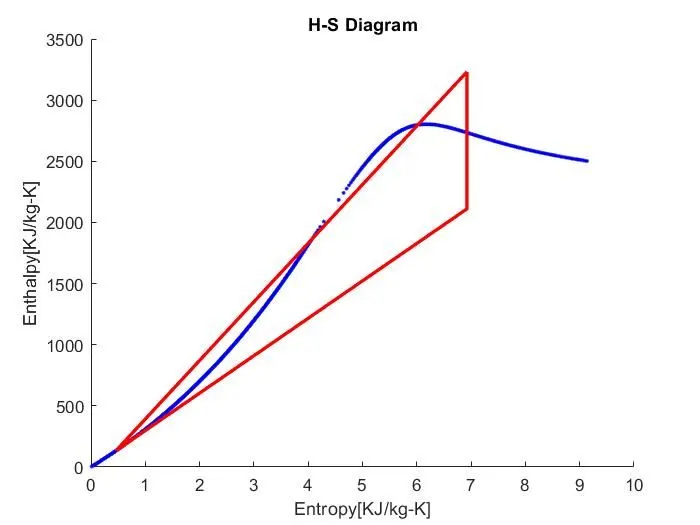
Output Plots:

Command Window:

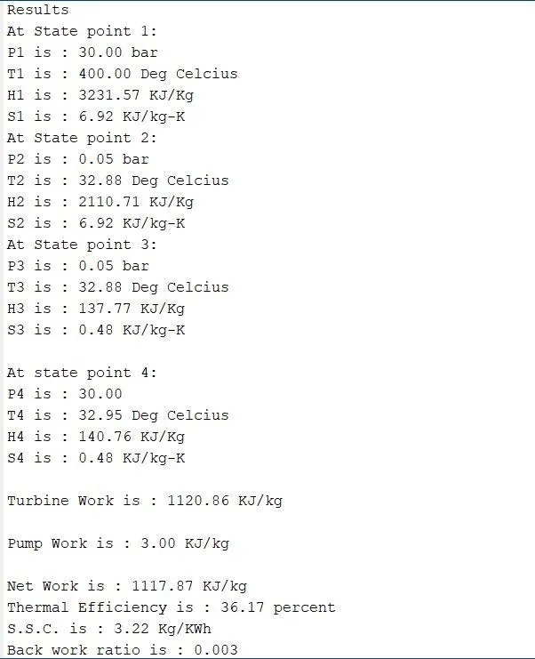
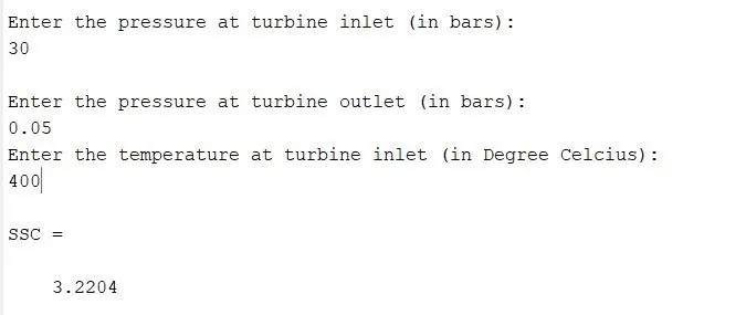
The command windows asks for inputs. 30, 0.05 and 400 are respective inputs by the user.

These are the required outputs presented systematically line by line in the command window: