Project 1 - Parsing NASA thermodynamic data

Aim:

To write a function that extracts the 14 coeffcients for 53 species from NASA's thermodynamic data and calculate the enthalpy, entropy and specific heats for all the species in the data file.

Objectives:

1. Write MATLAB code to extract the 14 coefficients.
2. Use the coefficients to find value of enthalpy, entropy and specific heat using the following formulas:
   • 
3. Use first 7 coeffs to find value for High temperature range and last 7 coeffs to find values for Low temperature range.
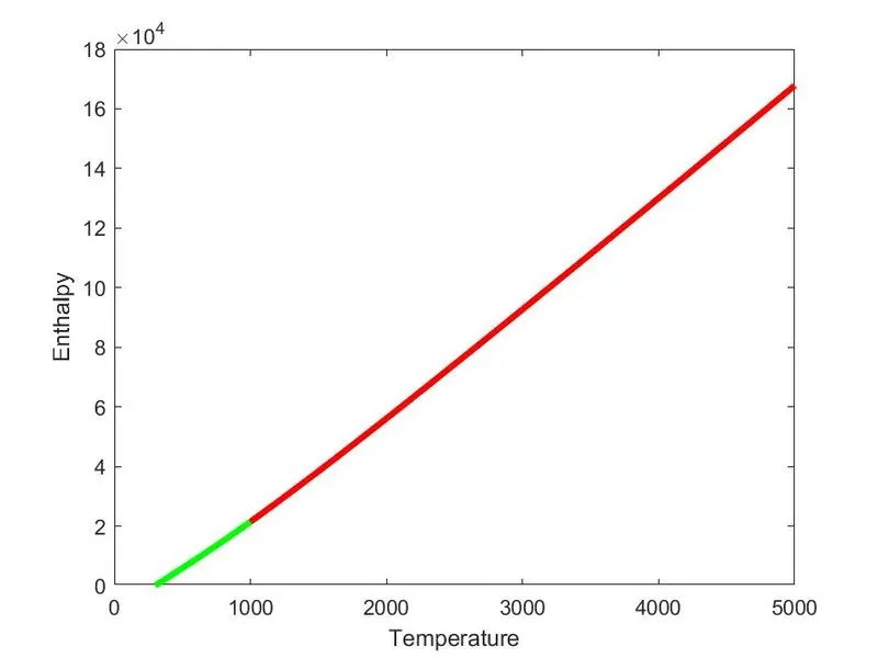
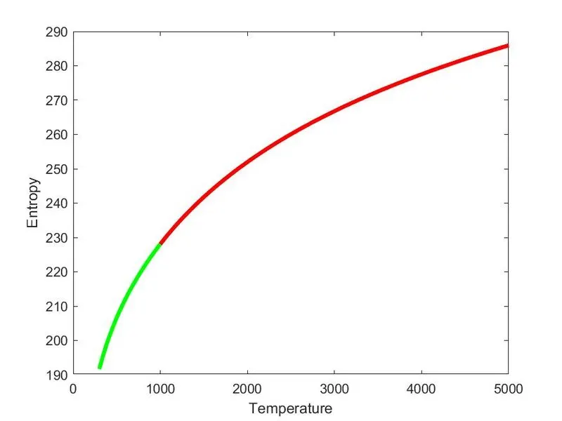
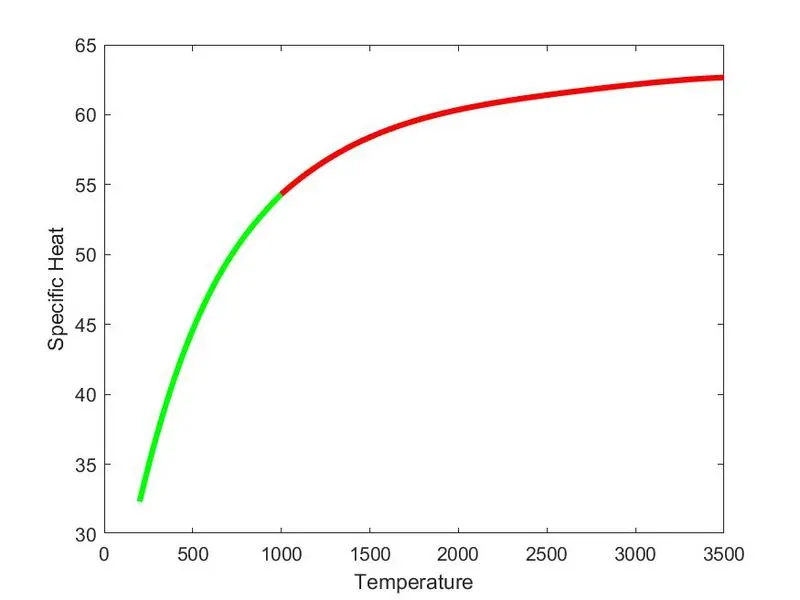
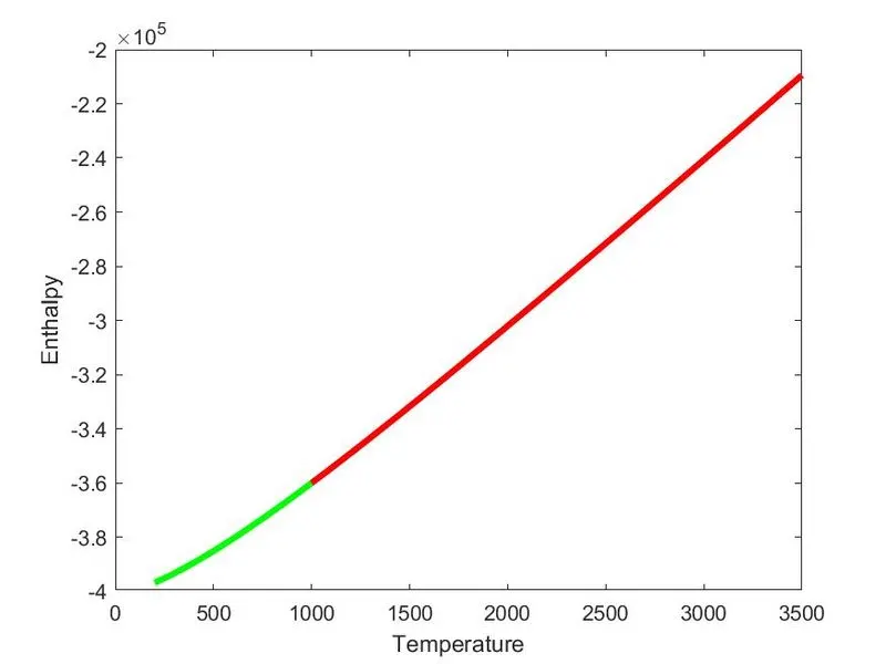
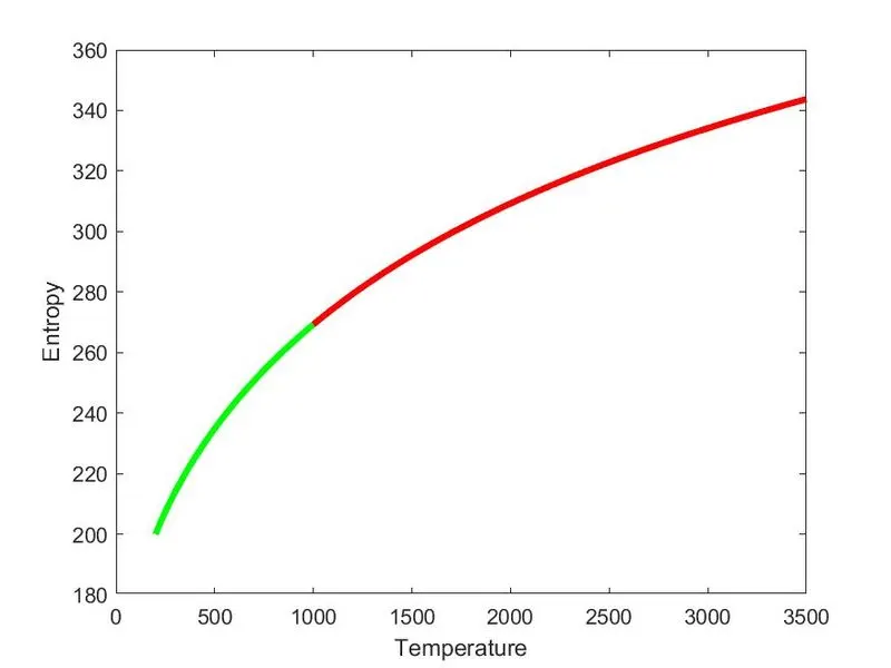
4. Plot enthalpy, entropy and specific heat vs temperature graphs for all species.
5. Write code to create individual folders for every specie and save the plots in the respective folders.

Code explaination:

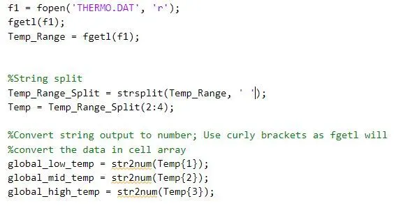
• Use fopen('data_file_name', 'r') to access data file. r represents read mode.
• Skip unwanted lines using: fgetl(data_file)
• Save 2nd line under variable: Temp_Range
  • strsplit(Temp_Range, ' ') will split the string using space as delimiter; Output is 3 strings for temperature range.
  • Save 3 trings in different variables. Use: str2num(Temp{1}) to convert string to number
    • strsplit creates a cell array. To access cell array use curly brackets {}.

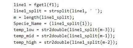
• Data for each specie is fitted in 4 lines. use fgetl to save line wise data in 4 variables.
  • First string of first line represents the specie name [save it under variable Specie_Name, 4th last string (represented by {m-3}) represents Low_temp for that specie, 3rd last string(represented by {m-2}) represents High_temp for that specie, 2nd last string(represented by {m-1}) represents Mid_temp for that specie [save values under respective variables].
  • str2double converts string to number with 2 points accuracy to facilitate calculations. Code to extract all 3:
  • 
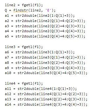
  • 2nd 3rd and 4th line contain 14 variables.
  • Use 'E' to pick individual coefficients; we save all the places of occurence of E under array 'Q'.
  • The code will collect data of 1st string till 3 strings after letter E; [(1:Q(1)+3]. For next coeff, use (Q(1)+4:Q(2)+3) and similarly for all 14 coeffs.
  • str2double converts string to number with 2 points accuracy to facilitate calculations.
  • Code to extract all 14:
  • 
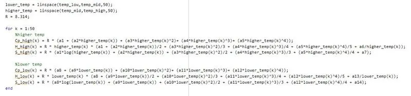
• Use the linspace command to split the temp range into 50 spaces.
  • Code the formulas in MATLAB to find Cp, H and S and run it for 50 times. so that a plot can be made. Two set of variables will be formed.
  • 
• mkdir(['file_location', Specie_Name]) will create a new folder in specified location with name of each specie as the complete code will run for 53 iterations and each time variable Specie_Name will have a spearate name.
  • cd(['file_location', Specie_Name]) will make the newly created folder of the name of specie as the current folder so that plots can be saved there.
  • 
• Use Plot command to plot the graphs of cp vs temp, H vs temp and S vs temp.
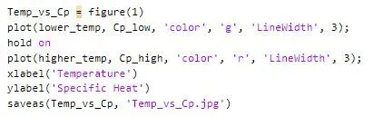
  • saveas(fig_name, 'Temp_vs_cp.jpg') will save the plot in the current folder with the name specified with the extension specified.
  • 
• Complete code is run 53 times as each run enterprets 4 lines of code, i.e. no. of lines contained by each specie and there are total 53 species

MATLAB code:

clear all
close all
clc

f1 = fopen('THERMO.DAT', 'r');
fgetl(f1);
Temp_Range = fgetl(f1);


%String split
Temp_Range_Split = strsplit(Temp_Range, ' ');
Temp = Temp_Range_Split(2:4);

%Convert string output to number; Use curly brackets as fgetl will
%convert the data in cell array
global_low_temp = str2num(Temp{1});
global_mid_temp = str2num(Temp{2});
global_high_temp = str2num(Temp{3});

for i = 1:3
    fgetl(f1);
end

for i = 1:53
    line1 = fgetl(f1);
    line1_split = strsplit(line1, ' ');
    m = length(line1_split);
    Specie_Name = (line1_split{1});
    temp_low = str2double(line1_split{m-3});
    temp_mid = str2double(line1_split{m-1});
    temp_high = str2double(line1_split{m-2});

    line2 = fgetl(f1);
    Q = findstr(line2, 'E');
    a1 = str2double(line2(1:Q(1)+3));
    a2 = str2double(line2(Q(1)+4:Q(2)+3));
    a3 = str2double(line2(Q(2)+4:Q(3)+3));
    a4 = str2double(line2(Q(3)+4:Q(4)+3));
    a5 = str2double(line2(Q(4)+4:Q(5)+3));

    line3 = fgetl(f1);
    a6 = str2double(line3(1:Q(1)+3));
    a7 = str2double(line3(Q(1)+4:Q(2)+3));
    a8 = str2double(line3(Q(2)+4:Q(3)+3));
    a9 = str2double(line3(Q(3)+4:Q(4)+3));
    a10 = str2double(line3(Q(4)+4:Q(5)+3));

    line4 = fgetl(f1);
    a11 = str2double(line4(1:Q(1)+3));
    a12 = str2double(line4(Q(1)+4:Q(2)+3));
    a13 = str2double(line4(Q(2)+4:Q(3)+3));
    a14 = str2double(line4(Q(3)+4:Q(4)+3));

lower_temp = linspace(temp_low,temp_mid,50);
higher_temp = linspace(temp_mid,temp_high,50);
R = 8.314;

for k = 1:50  
    %higher temp
    Cp_high(k) = R * (a1 + (a2*higher_temp(k)) + (a3*higher_temp(k)^2)+ (a4*higher_temp(k)^3)+ (a5*higher_temp(k)^4));
    H_high(k) = R * higher_temp(k) * (a1 + (a2*higher_temp(k))/2 + (a3*higher_temp(k)^2)/3 + (a4*higher_temp(k)^3)/4 + (a5*higher_temp(k)^4)/5 + a6/higher_temp(k));
    S_high(k) = R * (a1*log(higher_temp(k)) + (a2*higher_temp(k)) + (a3*higher_temp(k)^2)/2 + (a4*higher_temp(k)^3)/3 + (a5*higher_temp(k)^4)/4 + a7);

    %lower temp
    Cp_low(k) = R * (a8 + (a9*lower_temp(k)) + (a10*lower_temp(k)^2)+ (a11*lower_temp(k)^3)+ (a12*lower_temp(k)^4));
    H_low(k) = R * lower_temp(k) * (a8 + (a9*lower_temp(k))/2 + (a10*lower_temp(k)^2)/3 + (a11*lower_temp(k)^3)/4 + (a12*lower_temp(k)^4)/5 + a13/lower_temp(k));
    S_low(k) = R * (a8*log(lower_temp(k)) + (a9*lower_temp(k)) + (a10*lower_temp(k)^2)/2 + (a11*lower_temp(k)^3)/3 + (a12*lower_temp(k)^4)/4 + a14);
end

mkdir(['D:\A\Matlab\file parsing\plots\',Specie_Name]) ;
cd(['D:\A\Matlab\file parsing\plots\',Specie_Name]) ;

Temp_vs_Cp = figure(1)
plot(lower_temp, Cp_low, 'color', 'g', 'LineWidth', 3);
hold on
plot(higher_temp, Cp_high, 'color', 'r', 'LineWidth', 3);
xlabel('Temperature')
ylabel('Specific Heat')
saveas(Temp_vs_Cp, 'Temp_vs_Cp.jpg')

hold off


Temp_vs_H = figure(2)
plot(lower_temp, H_low, 'color', 'g', 'LineWidth', 3);
hold on
plot(higher_temp, H_high, 'color', 'r', 'LineWidth', 3);
xlabel('Temperature')
ylabel('Enthalpy')
saveas(Temp_vs_H, 'Temp_vs_H.jpg')

hold off


Temp_vs_S = figure(3)
plot(lower_temp, S_low, 'color', 'g', 'LineWidth', 3);
hold on
plot(higher_temp, S_high, 'color', 'r', 'LineWidth', 3);
xlabel('Temperature')
ylabel('Entropy')
saveas(Temp_vs_S, 'Temp_vs_S.jpg')

hold off


% mkdir
% cd
% saveas

clear('a1','a2','a3','a4','a5','a6','a7','a8','a9','a10','a11','a12','a13','a14','ans','i','k','line1','line2','line3','line4', 'line1_split','m','Q','Temp','Temp_Range','Temp_Range_Split')
end

Results:

Final output of the code, autosaving of plots in separate folders:

O2 Plot:

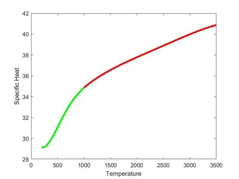
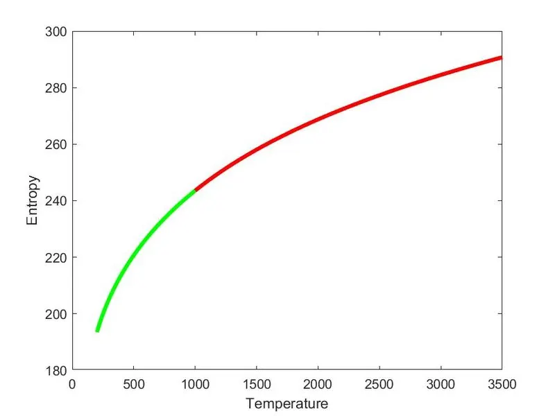
N2 Plots:

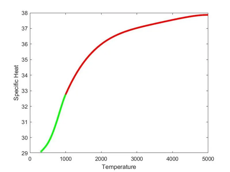
CO2 Plot:

Conclusion:

Information from complex data files can be extracted, stored and be further used to perform calculations by using file parsing functions and techniques.