Week 4.1 - Genetic Algorithm

GENETIC ALGORITHM

Objective

• To develop a code in MATLAB to optimize the stalagmite function and find the global maxima of the function.
• To explain the concept of genetic algorithm in your own words and also explain the syntax for gain MATLAB.
• And to plot the graphs for all 3 studies and for F maximum vs no. of iterations.

Principle

Genetic Algorithms (GAs) are adaptive heuristic search algorithms that belong to the larger part of evolutionary algorithms. Genetic algorithms are based on the ideas of natural selection and genetics. These are intelligent exploitation of random search provided with historical data to direct the search into the region of better performance in solution space. They are commonly used to generate high-quality solutions for optimization problems and search problems.

Genetic algorithms simulate the process of natural selection which means those species who can adapt to changes in their environment are able to survive and reproduce and go to the next generation. In simple words, they simulate “survival of the fittest” among individuals of consecutive generations for solving a problem. Each generation consists of a population of individuals and each individual represents a point in search space and possible solution. Each individual is represented as a string of character/integer/float/bits. This string is analogous to the Chromosome.

Foundation of Genetic Algorithms

Genetic algorithms are based on an analogy with the genetic structure and behavior of chromosomes of the population. Following is the foundation of GAs based on this analogy –

1. Individuals in the population compete for resources and mate
2. Those individuals who are successful (fittest) then mate to create more offspring than others
3. Genes from the “fittest” parent propagate throughout the generation, that is sometimes parents create offspring which is better than either parent.
4. Thus, each successive generation is more suited for their environment.

Search space

The population of individuals is maintained within search space. Each individual represents a solution in search space for the given problem. Each individual is coded as a finite length vector (analogous to chromosome) of components. These variable components are analogous to Genes. Thus a chromosome (individual) is composed of several genes (variable components).

Fitness Score

A Fitness Score is given to each individual which shows the ability of an individual to “compete”. The individual having optimal fitness score (or near-optimal) is sought.

The GAs maintains the population of n individuals (chromosome/solutions) along with their fitness scores. The individuals having better fitness scores are given more chances to reproduce than others. The individuals with better fitness scores are selected who mate and produce better offspring by combining chromosomes of parents. The population size is static so the room has to be created for new arrivals. So, some individuals die and get replaced by new arrivals eventually creating a new generation when all the mating opportunity of the old population is exhausted. It is hoped that over successive generations better solutions will arrive while at least fit die.

Each new generation has on average more “better genes” than the individual (solution) of previous generations. Thus, each new generations have better “partial solutions” than previous generations. Once the offspring produced has no significant difference from offspring produced by previous populations, the population is converged. The algorithm is said to be converted to a set of solutions for the problem.

Operators of Genetic Algorithms

Once the initial generation is created, the algorithm evolves the generation using the following operators –
1) Selection Operator: The idea is to give preference to the individuals with good fitness scores and allow them to pass their genes to successive generations.
2) Crossover Operator: This represents mating between individuals. Two individuals are selected using a selection operator and crossover sites are chosen randomly. Then the genes at these crossover sites are exchanged thus creating a completely new individual (offspring). For example –

3) Mutation Operator: The key idea is to insert random genes in offspring to maintain the diversity in the population to avoid premature convergence. For example –

The whole algorithm can be summarized as –

1) Randomly initialize populations p

2) Determine fitness of the population

3) Until convergence repeat:

1. a) Select parents from population
2. b) Crossover and generate a new population
3. c) Perform mutation on new population
4. d) Calculate fitness for new population

Solution Procedure

The process of natural selection starts with the selection of the fittest individuals from a population. They produce offspring which inherit the characteristics of the parents and will be added to the next generation.

In a genetic algorithm, a population of candidate solutions (called individuals, creatures, or phenotypes) to an optimization problem is evolved toward better solutions. Each candidate solution has a set of properties (its chromosomes or genotype) that can be mutated and altered; traditionally, solutions are represented in binary as strings of 0s and 1s, but other encodings are also possible.[3]

The evolution usually starts from a population of randomly generated individuals, and is an iterative process, with the population in each iteration called a generation. In each generation, the fitness of every individual in the population is evaluated; the fitness is usually the value of the objective function in the optimization problem being solved.

The more fit individuals are stochastically selected from the current population, and each individual's genome is modified (recombined and possibly randomly mutated) to form a new generation. The new generation of candidate solutions is then used in the next iteration of the algorithm. Commonly, the algorithm terminates when either a maximum number of generations has been produced, or a satisfactory fitness level has been reached for the population.

This notion can be applied to a search problem. We consider a set of solutions for a problem and select the set of best ones out of them.

Generally, five phases are considered in a genetic algorithm:

1. Initial population
2. Fitness function
3. Selection
4. Crossover
5. Mutation

A genetic algorithm (GA) is a method for solving both constrained and unconstrained optimization problems based on a natural selection process that mimics biological evolution. The algorithm repeatedly modifies a population of individual solutions. At each step, the genetic algorithm randomly selects individuals from the current population and uses them as parents to produce the children for the next generation. Over successive generations, the population “evolves” toward an optional solution.

We can apply the genetic algorithm to solve problems that are not well suited for standard optimization algorithms, including problems in which the objective function is discontinuous, non-differentiable, stochastic, or highly non-linear.

A genetic algorithm differs from a classical, derivative-based, optimization algorithm in two main ways:

Classical Algorithm	Genetic Algorithm
It generates a point at each iteration. The sequence of points approaches an optimal solution.	Generates a population of points at each iteration. The best point in the population approaches an optimal solution.
Selects the next point in the sequence by a deterministic computation.	Selects the next population by computation which uses random number generators.

Working of Genetic Algorithm

• The algorithm begins by creating a random initial population.
• The algorithm creates a sequence of new populations. At each step, the algorithm uses the individuals in the current generation to create the next population. To create a new population, the algorithm performs the following steps: -
• Scales the raw fitness scores to convert them into a more usable range of values. These scaled values are called expectation values.
• Selects members, called parents, based on their expectations.
• Some of the individuals in the current population that have lower fitness are chosen as elite. These elite individuals are passed to the next population.
• Produces children from their parents. Children are produced either by making random changes to a single parent mutation by combining the vector entries of a pair of parents’ crossovers.
• Replaces the current population with the children ton from the next generation.

Scores each member of the current population by computing its fitness value. These values are called raw fitness scores.

• The algorithm stops when one of the stopping criteria is met.

Why use Genetic Algorithms

• They are Robust
• Provide optimization over large space state.
• Unlike traditional AI, they do not break on a slight change in input or presence of noise

Advantages of GAs

GAs has various advantages which have made them immensely popular. These include −

• Does not require any derivative information (which may not be available for many real-world problems).
• Is faster and more efficient as compared to the traditional methods.
• Has very good parallel capabilities.
• Optimizes both continuous and discrete functions and also multi-objective problems.
• Provides a list of “good” solutions and not just a single solution.
• Always gets an answer to the problem, which gets better over time.
• Useful when the search space is very large and there are a large number of parameters involved.

Limitations of GAs

Like any technique, GAs also suffers from a few limitations. These include −

• GAs is not suited for all problems, especially problems that are simple and for which derivative information is available.
• The fitness value is calculated repeatedly which might be computationally expensive for some problems.
• Being stochastic, there are no guarantees on the optimality or the quality of the solution.
• If not implemented properly, the GA may not converge to the optimal solution.

Application of Genetic Algorithms

Genetic algorithms have many applications, some of them are –

• Recurrent Neural Network
• Mutation testing
• Codebreaking
• Filtering and signal processing
• Learning fuzzy rule base etc

Code for Stalagmite function

function[f] = stalagmite(input_vector) %function to perform the task of stalagmite function

%Initializing x and y input

x=input_vector(1);	% To initialize the first column
y=input_vector(2);	% To initialize the second column

%term X1 is equation for f1_x and term Y1 is equation for f1_y

termX1 = (sin(5.1*pi*x +0.5))^6;		%Initializing term according to the equation
termY1 = (sin(5.1*pi*y +0.5))^6;		%Initializing term according to the equation

%term X2 is the equation for f2_x and term Y2 is the equation for f2_y

termX2 = exp(-4*log(2)*((x-0.0667)^2/0.64));	%Initializing term according to the equation
termY2 = exp(-4*log(2)*((y-0.0667)^2/0.64));	%Initializing term according to the equation

f = -(termX1*termY1*termX2*termY2);		%Calculating the value according to the stalagmite function

end

Code for genetic algorithm

clear           % To clear all the workspace variables
close all       % To close all output window
clc             % To clear all the command window

%Defining search space
x = linspace(0,0.6,150);    % Linspace command is used to generate 150 values between 0 and 0.6
y = linspace(0,0.6,150);    % Linspace command is used to generate 150 values between 0 and 0.6
num_case = 50;

%Creating a 2D mesh
[xx,yy] = meshgrid(x,y);    % Used to create a diimensional array

%Evaluating the stalagmite function
for i = 1:length(xx)        % For execution of the statements in loop till length(xx)
	for j= 1:length(yy)     % For execution of the statements in loop till length(yy)
	input_vector(1)=xx(i,j);    % Initializing the array rows and coloumns
	input_vector(2)=yy(i,j);    % Initializing the array rows and coloumns
    f(i,j) = stalagmite(input_vector);  % calls the stalagmite function to get the value by passing input vector
    end     % to terminate the for loop
end         % to terminate the for loop

surfc(xx,yy,f)      % To generate surface plot
xlabel('x value')   % Labeling the x value
ylabel('y value')   % Labeling the y value
shading interp      % To remove gridlines on the plot
[inputs, fval] = ga(@stalagmite,2)  % Syntax for genetic algorithm

%Study 1-Statistical behaviour
tic                 % command to check how much does it take to complete
for i = 1:num_case  % For execution of for loop till 50 times
[inputs,fopt(i)] = ga(@stalagmite,2);   % Syntax for genetic algorithm
xopt(i) = inputs(1);    % To initialize the x optimum value
yopt(i) = inputs(2);    % To initialize the y optimum value
end                     % to terminate the for loop

Study1_time = toc  % command to check how much does it take to complete
figure(1)           % To generate a figure window
subplot(2,1,1)      % To have multiple plot inside the same figure window
hold on             % To change the hold state to on
surfc(x,y,-f)       % To generate the surface plot
xlabel('x value')   % Labeling the x value
ylabel('y value')   % Labeling the y value
shading interp      % To remove gridlines on the plot

plot3(xopt,yopt,-fopt,'marker','o','markersize',5,'markerfacecolor','r') % To plot optimum value that ga predict over the 50 studies
title('Unbound inputs') % To give title to the plot
subplot(2,1,2)          % To have multiple plot inside the same figure window
plot(-fopt)         
xlabel('Iterations')        % Labeling the x value
ylabel('Function minimum')  % Labeling the y value

tic     % command to check how much does it take to complete
%Study 2 for the optimization
for i = 1:num_case          % For execution of for loop till 50 times
	[inputs,fopt(i)]=ga(@stalagmite,2,[],[],[],[],[0:0],[0.5:0.5]); % syntax for ga
xopt(i) = inputs(1);        % To initialize the x optimum value
yopt(i) = inputs(2);        % To initialize the y optimum value
end                         % to terminate the for loop
Study2_time = toc          % command to check how much does it take to complete
figure(2)                   % To generate a figure window
subplot(2,1,1)              % To have multiple plot inside the same figure window
hold on                     % To change the hold state to on
surfc(x,y,-f)                % To generate the surface plot
xlabel('x value')           % Labeling the x value
ylabel('y value')           % Labeling the y value
shading interp              % To remove gridlines on the plot

plot3(xopt,yopt,-fopt,'marker','o','markersize',5,'markerfacecolor','r') % To plot optimum value that ga predict over the 50 studies
title('Bound inputs')       % To give title to the plot
subplot(2,1,2)              % To have multiple plot inside the same figure window
plot(-fopt)                 
xlabel('Iterations')        % Labeling the x value
ylabel('Function maximum')  % Labeling the y value


options = optimoptions(@ga);    % To set the population size minimize the non default options
options = optimoptions(options,'populationsize',360);
tic                             % command to check how much does it take to complete

%Study 3 for the optimization

for i = 1:num_case              % For execution of for loop till 50 times
	[inputs , fopt(i)]=ga(@stalagmite,2,[],[],[],[],[0:0],[1:1],[],[],options);
xopt(i) = inputs(1);            % To initialize the x optimum value
yopt(i) = inputs(2);            % To initialize the y optimum value
end                             % to terminate the for loop

Study3_time = toc              % command to check how much does it take to complete
figure(3)                       % To generate a figure window
subplot(2,1,1)                  % To have multiple plot inside the same figure window
hold on                         % To change the hold state to on
surfc(x,y,-f)                    % To generate the surface plot
xlabel('x value')               % Labeling the x value
ylabel('y value')               % Labeling the y value
shading interp                  % To remove gridlines on the plot

plot3(xopt,yopt,-fopt,'marker','o','markersize',5,'markerfacecolor','r') % To plot optimum value that ga predict over the 50 studies
title('Bound inputs')           % To give title to the plot
subplot(2,1,2)                  % To have multiple plot inside the same figure window
plot(-fopt)
xlabel('Iterations')            % Labeling the x value
ylabel('Function maximum')      % Labeling the x value

Outputs

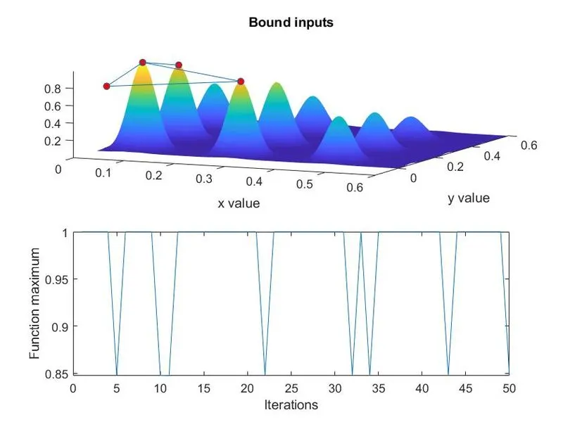
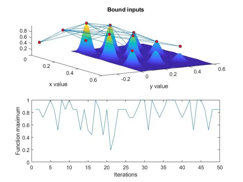
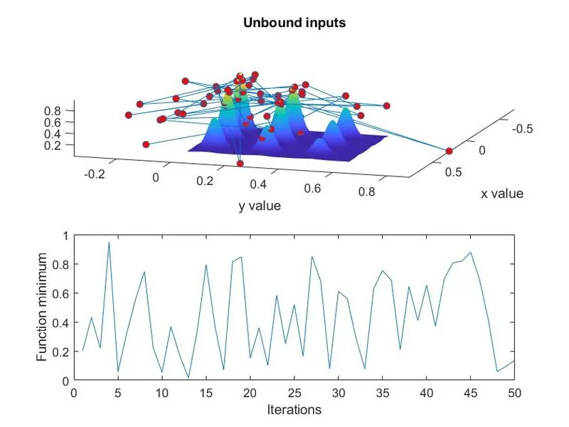
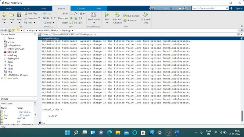
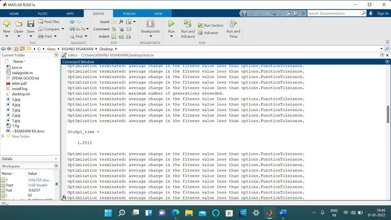
Study time for 1^st study

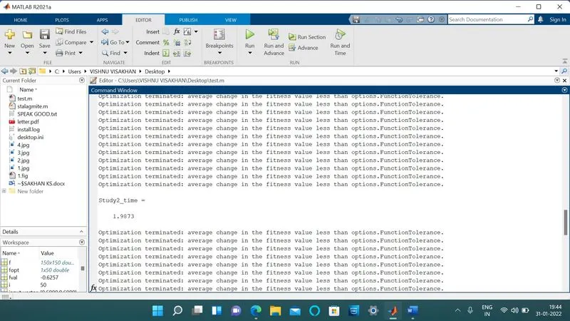
Study time for 2^nd study

Study time for 3^rd study

Errors faced

Mentioned in the document attached.

Conclusion

• Study time for 1^st study was 1.2158sec
• Study time for 2^nd study was 1.9873sec
• Study time for 3^rd study was 9.6493sec
• The stalagmite equation was multiplied by (-1) to generate a downward stalagmite.
• F=-f so that the minimum value of f is the maximum value for f and vice versa.

Reference

• Genetic Algorithm - MATLAB & Simulink (mathworks.com)
• Genetic Algorithms - GeeksforGeeks
• Genetic Algorithms - Quick Guide (tutorialspoint.com)
• https://en.wikipedia.org/wiki/List_of_genetic_algorithm_applications
• https://en.wikipedia.org/wiki/Genetic_algorithm
• https://www.doc.ic.ac.uk/~nd/surprise_96/journal/vol1/hmw/article1.html