Week 4.1 - Genetic Algorithm

Write a code in MATLAB to optimise the stalagmite function and find the GLOBAL MAXIMA of the function

THEORY :

GENETIC ALGORITHM :

• Genetic Algorithm (GA) is a search-based optimization technique based on the principles of Genetics and Natural Selection.
• It is frequently used to find optimal or near-optimal solutions to difficult problems which otherwise would take a lifetime to solve.
• It is frequently used to solve optimization problems, in research, and in machine learning.
• There are three main components in genetic algorithms
  1. Crossover
  2. Mutation
  3. Selection of the fittest.
• The genetic algorithm can be applied to solve a variety of optimization problem that are not well suited for standard optimization algorithms, Including problems in which the objective function is discontinous, non-differentiable , stochastic or highly nonlinear.

SYNTAX OF GA :

• x = ga(fun,nvars) finds a local unconstrained minimum, x, to the objective function, fun.nvars is the dimensio (number of design variables) of fun.
• x = ga(fun,nvars,A,b) finds a local minimum x to fun, subject to the linear inequalities `A*x<=b`. ga evaluates the matrix product A*x as if x is transposed (A*x').
• x = ga(fun,nvars,A,b,Aeq,beq) finds a local minimum x to fun, subject to the linear equalities Aeq*x = beq and A*x`<=`b. (Set A=[ ] and b=[ ] if no linear inequalities exist.) ga evaluates the matrix product aeq*x as if x is transposed (Aeq*x')
• x = ga(fun,nvars,A,b,Aeq,beq,lb,ub) defines a set of lower and upper bounds on the design variables x, so that a solution is found in the range 1b`<=` x `<=`ub. (Set Aeq=[ ] and beq=[ ] if no linear equalities exist.)
• x = ga(fun,nvars,A,b,Aeq,beq,lb,ub,nonlcon) subjects the minimization to the constraints defined in nonlcon. The function nonlcon accepts x and returns vectors c and Ceq, representing the nonlinear inequalities and equalities respectively. ga minimizes the fun such that c(x) `<=`0 and Ceq(x) = 0 (Set 1b = [ ] and ub=[ ] if no bounds exist.)
• x = ga(fun,nvars,A,b,Aeq,beq,lb,ub,nonlcon,options) minimizes with the default optimization parameters replaced by values in option. (Set nonlcon=[ ] if no nonlinear constraints exist.) Create options using optimoptions.
• x = ga(fun,nvars,A,b,Aeq,beq,lb,ub,nonlcon,intcon,options) requires that the variables listed in intcon take integer values.
• x = ga(problem) finds the minimum for problem, a structure described in problem.
• [x,fval] = ga(__), for any previous input arguments, also returns fval, the value of the fitness function at x.
• [x,fval,exitflag,output] = ga(__) also returns exitflag, an integer identifying the reason the algorithm terminated, and outpit, a structure that contains output from each generation and other information about the performance of the algorithm.
• [x,fval,exitflag,output,population,scores] = ga(__) also returns a matrix population, whose rows are the final population, and a vector scores, the scores of the final population.

GOVERNING EQUATIONS :

• Stalagmite Function `f(x,y) = f1,xf2,xf1,yf2,y`
• Where,
  • `f1,x = [sin(5.1pix + 0.5)]^6`
  • `f1,y = [sin(5.1pix + 0.5)]^6`
  • `f2,x = exp[-4ln(2)frac{(x-0.0667)^2}{0.64}]`
  • `f2,y = exp[-4ln(2)frac{(y-0.0667)^2}{0.64}]`

MAIN PROGRAM :

clear all
close all
clc

%Defining search space
x = linspace(0,0.6,150);
y = linspace(0,0.6,150);

%Iteration Count
num_cases = 500;

% creating a 2Dimensional mesh
[xx, yy] = meshgrid(x,y);

%Evaluating the stalagmite function
for i=1:length(xx)
    for j=1:length(yy)
        input_vector(1)=xx(i,j);
        input_vector(2)=yy(i,j); 
        f(i,j) =stalagmite(input_vector);
    end
end

%Study=1 Unbounded
tic
for i = 1: num_cases
    [results,fopt(i)]=ga(@stalagmite,2)
    opt_x(i) = results(1);
    opt_y(i) = results (2);
end
study_time1=toc
figure(1)
subplot(2,1,1)
surf(xx,yy,-f)
hold on

%remove gridlines on the 3D surface 
shading interp

plot3(opt_x,opt_y,-fopt,'marker','o','MarkerSize',5,'MarkerFaceColor','b')
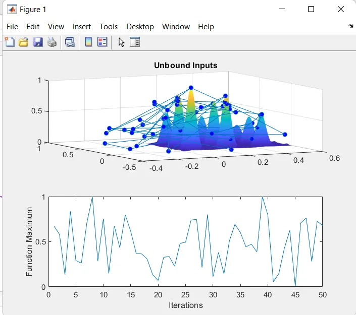
title('Unbound Inputs')
subplot(2,1,2)
plot(-fopt)
xlabel('Iterations')
ylabel('Function Maximum')
title('Unbounded Inputs')

%study 2 - Bounded
tic
for i=1:num_cases
    [results,fopt(i)] = ga(@stalagmite,2,[],[],[],[],[0;0],[0.6;0.6]);
    xopt(i) = results(1);
    yopt(i) = results(2);
end
study_time2=toc
figure(2)
subplot(2,1,1)
surf(xx,yy,-f)
shading interp
hold on
plot3(xopt,yopt,-fopt,'marker','o','MarkerSize',5,'MarkerFaceColor','b')
subplot(2,1,2)
plot(-fopt)
xlabel('Iteration')
ylabel('Function Maximum')
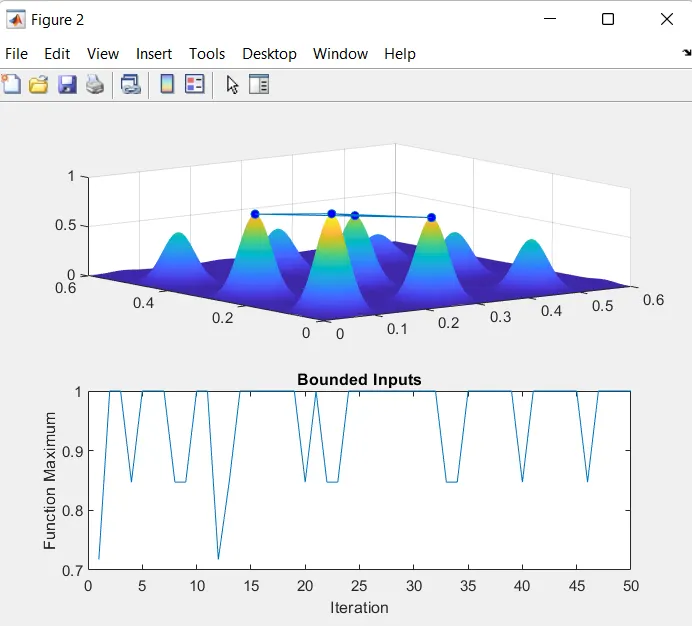
title('Bounded Inputs')

%Study 3 Increased intial population

tic
options = optimoptions('ga');
options = optimoptions(options,'PopulationSize',250);

for i=1:num_cases
    [results,fopt(i)] = ga(@stalagmite,2,[],[],[],[],[0;0],[0.6,0.6],[],[],options);
    xopt(i)= results(1);
    yopt(i)= results(2);
end

study_time3 = toc
figure(3)
subplot(2,1,1)
surf(xx,yy,-f)
shading interp
hold on
plot3(xopt,yopt,-fopt,'marker','o','MarkerSize',5,'MarkerFaceColor','b')
subplot(2,1,2)
plot(-fopt)
xlabel('Iteration')
ylabel('Function Maximum')
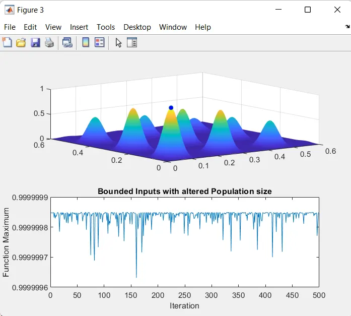
title('Bounded Inputs with altered Population size')

STALAGMITE FUNCTION PROGRAM :

function [f] = stalagmite(input_vector)
x = input_vector(1);
y = input_vector(2);

 a = (sin(5.1*pi*x + 0.5))^6;
 b = (sin(5.1*pi*y + 0.5))^6;
 c = exp(-4*log(2)*(x-0.0667)^2/0.64);
 d = exp(-4*log(2)*(y-0.0667)^2/0.64);

[f] = -(a*b*c*d);
end

STEP-WISE EXPLANATION OF PROGRAM :

• First start with clear all , close all & clc commands,
• then define the search space,
• now provide the iteration count and create a 2D mesh using meshgrid command,
• then create stalagmite function program in seperate scipte and define the formula which is explain in Govening equation,
• then Evaluting the stalagmite function using for loop command,
• this program is divied in three studys, Unbounded inputs , bounded inputs & Increase in intial population respectively,
• first study deals with unbounded inputs, expanding the boundary where results can be obtained,
• second study brings in the aspect of bounded input providing the better solution,
• and the third study create a appriciable platform to detemine the exact solution,
• plot all the studies so we get the clear view of the results.

ERROR & SOLUTION :

• options = prepareoptionsforsolvererror an error found while running the program, after some reaserch found that pc don't have a 'Globel optimization Tool box' . because of these the GA is not runninng in MATLAB. So install these tool box in MATLAB throug MATLAB setup and it's Solve the error.(forgot to take Screenshot of an error)

OUTPUT :

• Study 1 :

• Study 2 :

• Study 3 :