Project 2 - Rankine cycle Simulator

AIM : Rankine Cycle Using MATLAB

OBJECTIVE :

• Calculate each state points of rankine cycle(any type of your choice) based on user inputs.
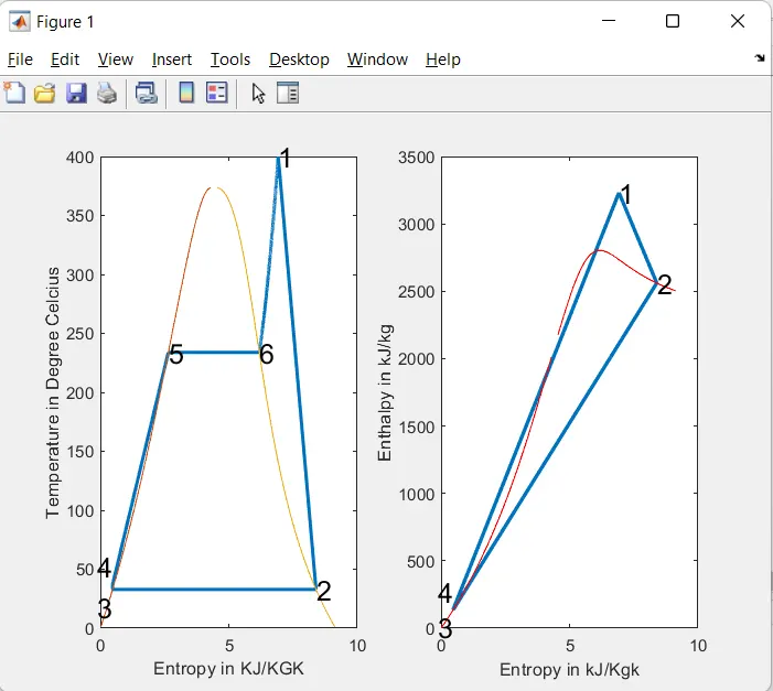
• Plot the T-S & H-S diagram for the given set of input
• Calculate Efficiency.

THEORY :

The Rankine cycle is an idealized thermodynamic cycle of a heat engine that converts heat into mechanical work while undergoing a phase change. It is an idealized cycle in which friction losses in each of four components are neglected. The heat is supplied externally to a closed loop, which usually uses water as the working fluid.

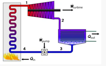
• Four Componets of Rankine Cycle :

1. Pump
2. Boiler
3. Turbine
4. Condenser

• Four Processes of the Rankine Cycle :

• 1-2 Isentropic Expantion : Turbine (1-2)
  • Superheted steam enters into the turbine and expands isentropically resulting in the production of work
  • The Shaft of the turbine is connected to the generator. This results in the production of electricity
  • Work Produce by turbine,

`W_T = m(h_1 - h_2)K`

• 2-3 Constant Pressure Heat Rejection : Condensor (2-3)
  
  • The expanded vapour is then passed through a condensor, where it gets condensed and converts into liqiud again
  • this liquid is again pumped to the boiler.

`Q_r = m(h_2 - h_3 )K`

• 3-4 Isentripic Compression by the Pump : Pump (3-4)
  • The Water enters into pump in a saturated state.
  • Then the liquid is compressed isentropically until it meets the boiler pressure
  • Work done by Pump is `W_P = m(h_3 - h_4)K`

• 4-1 Constant Pressure Heat Addition : Boiler (4-1)
  • The Water enters into boiler as compressed and leaves as superheated from the boiler.
  • Thus the Phase Change from liquid to vapour
  • The heat supplied by the bolier is,

`Q_b = m(h_1 - h_4 )K`

• The Efficiency of the steam Cycle is given by

`eta = W_n/Q_1 =frac{ W_T - W_P}{Q_1}`

• Applying the SFEE to all the process, neglecting the Friction losses and changes in kinrtic & Potencial Energy.
  • `Q_1 = h_1 - h_4` (Boiler )
  • `W_T = h_1 - h_2` (Turbine)
  • `Q_2 = h_2 - h_3` (Condenser)
  • `W_p = h_4 - h_3` (Pump)

• The Cpacity of the Steam Plant is often expresssed interms of SSC

`S.S.C = 3600/W_n frac{kg}{kWh}`

Required Input :

Turbine Inlet Temperature = 400 C

Turbine Inlet Pressure = 30 bar

Turbine Outlet Pressure = 0.05 bar = Condenser Inlet Pressure

MATLAB PROGRAM :

close all
clear all
clc

%Print Process Discription
fprintf('1-2 Isobaric Heat Transfer\n')
fprintf('2-3 Isentropic Expantion\n')
fprintf('3-4 Isobaric heat Rejection\n')
fprintf('4-1 Isentropic Compression\n')

%Step 1 : Enter Inputs
p1 = input('Enter the Pressure at the Turbine Inlet (in Bar):');
T1 = input('Enter the Temperature at the Turbine Inlet (in Degree Celcius):');
p2 = input('Enter the Pressure at the  Condensor (in Bar):');

% Step 2 : Calculate Each State Point values
% State Point 1
h1 = XSteam('h_pt',p1,T1);
s1 = XSteam('s_pt',p1,T1);

% State Point 2
s2 = s1;
sf2 = XSteam('sL_p',p2);
sg2 = XSteam('sV_p',p2);
hf2 = XSteam('hL_p',p2);
hg2 = XSteam('hV_p',p2);
s2 = sg2;
h2 = hg2;
T2 = XSteam('T_hs',h2,s2);

% State Point 3 
T3 = T2;
p3 = p2;
s3 = XSteam('sL_T',T3);
h3 = XSteam('hL_T',T3);
v3 = XSteam('vL_p',p2);

% State Point 4
p4 = p1;
s4 = s3;
Cp4 = XSteam('Cp_ps',p4,s4);
Cv4 = XSteam('Cv_ps',p4,s4);
gamma = Cp4/Cv4;
r = (gamma-1)/gamma;
T4 = T3*(p4/p3)^r;

% Step 3 : Calculate other output values
Wt = h1-h2;
Wp = v3*(p1-p2)*100;
h4 = Wp+h3;
W_net = Wt-Wp;
Qs = h1-h4;
N_per = (W_net/Qs)*100;
steam_rate = 3600/(Wt-Wp);

% Step 4 : state point 5 & 6 Which help in plotting
T5 = XSteam('Tsat_p',p1);
T6 = T5;
s5 = XSteam('sL_p',p1);
s6 = XSteam('sV_p',p1);
h5 = XSteam('hL_p',p1);
h6 = XSteam('hV_p',p1);

% Step 5 : print all state point values to show
fprintf('At State point 1:\nP1 is : %4.2f Bar\nT1 is : %4.2f Degree Celcius\nH1 is : %4.2f kJ/Kg\nS1 is : %4.2f KJ/kgk\n\n',p1,T1,h1,s1)
fprintf('At State point 2:\nP2 is : %4.2f Bar\nT2 is : %4.2f Degree Celcius\nH2 is : %4.2f kJ/Kg\nS2 is : %4.2f KJ/kgk\n\n',p2,T2,h2,s2)
fprintf('At State point 3:\nP3 is : %4.2f Bar\nT3 is : %4.2f Degree Celcius\nH3 is : %4.2f kJ/Kg\nS3 is : %4.2f KJ/kgk\n\n',p3,T3,h3,s3)
fprintf('At State point 4:\nP4 is : %4.2f Bar\nT4 is : %4.2f Degree Celcius\nH4 is : %4.2f kJ/Kg\nS4 is : %4.2f KJ/kgk\n\n',p4,T4,h4,s4)
fprintf('Wt is : %4.2f KJ/kg\nWp is : %4.2f KJ/kg\nWet is : %4.2f kJ/kg\nNtherm is : %4.2f percent\nS.S.C is : %4.2f kg/kWh',Wt,Wp,W_net,N_per,steam_rate)

% Step 6 : plot T-S Diagram
subplot(1,2,1)
T_rankine = linspace(T5,T1,5000);
for i = 1:length(T_rankine)
    s_rankine(i)=XSteam('s_pT',p1,T_rankine(i));
end

plot([s1 s2 s3 s4 s5 s6 s_rankine],[T1 T2 T3 T4 T5 T6 T_rankine],'LineWidth',2);
hold on
T_curve = linspace(1,400,500);
for i=1:length(T_curve)
    s_l(i) = XSteam('sL_T',T_curve(i));
    s_v(i) = XSteam('sV_T',T_curve(i));
    h_l(i) = XSteam('hL_T',T_curve(i));
    h_v(i) = XSteam('hV_T',T_curve(i));
end

plot(s_l,T_curve);
plot(s_v,T_curve);
text(s1,T1,'1','FontSize',15)
text(s2,T2,'2','FontSize',15)
text(s3,T3,'3','FontSize',15,'HorizontalAlignment','right','VerticalAlignment','top')
text(s4,T4,'4','FontSize',15,'HorizontalAlignment','right','VerticalAlignment','bottom')
text(s5,T5,'5','FontSize',15)
text(s6,T6,'6','FontSize',15)
xlabel('Entropy in KJ/KGK');
ylabel('Temperature in Degree Celcius');

% Step 7 : plot H-S Diagram
subplot(1,2,2)
plot([s1 s2 s3 s4 s1],[h1 h2 h3 h4 h1],'LineWidth',2)
hold on
plot(s_v,h_v,"Color",'r')
plot(s_l,h_l,'Color','r')
text(s1,h1,'1','FontSize',15)
text(s2,h2,'2','FontSize',15)
text(s3,h3,'3','FontSize',15,'HorizontalAlignment','right','VerticalAlignment','top')
text(s4,h4,'4','FontSize',15,'HorizontalAlignment','right','VerticalAlignment','bottom')
xlabel('Entropy in kJ/Kgk')
ylabel('Enthalpy in kJ/kg')

STEP-WISE EXPLANATION OF PROGRAM :

• The program start with Clear all , Close all , clc commands,
• Define the innput variable p1 ,T1, p2 Whose values are provide manually in commad window while simulation process,
• Then Calculate each state point values with the help of XSteam file and respective Formulas,
• In State point 1 Values of Enthalpt & Entropy are extracted as a function of pressure & temperature,
• State point 2 is a condenser inlet where the high-pressure steam is converted into low-pressure water and hence dryness fraction,
• state point 3 the water is condensed back to its saturation temperature and fed to the pump, This temperature of water at the exit of the condeser and entry of pump is the same,
• state point 4 this is constant pressure heat addition, hence pressure is equal to p1, but the temperature increases on heating at constant pressure & volume,
• Then define state point 5 & 6 values to plot rankine cycle detail,
• then calculate other outputs like, work done, heat evolved , S.S.C etc... bt basic formulas
• now plot the T-S & H-S diagram,
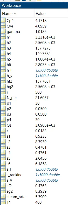
• Results of the Rankine cycle simulation is displayed over command window using fprintf command.

Results :

Command Window :

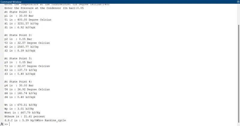
WorkSpace :

ERROR & SOLUTION :

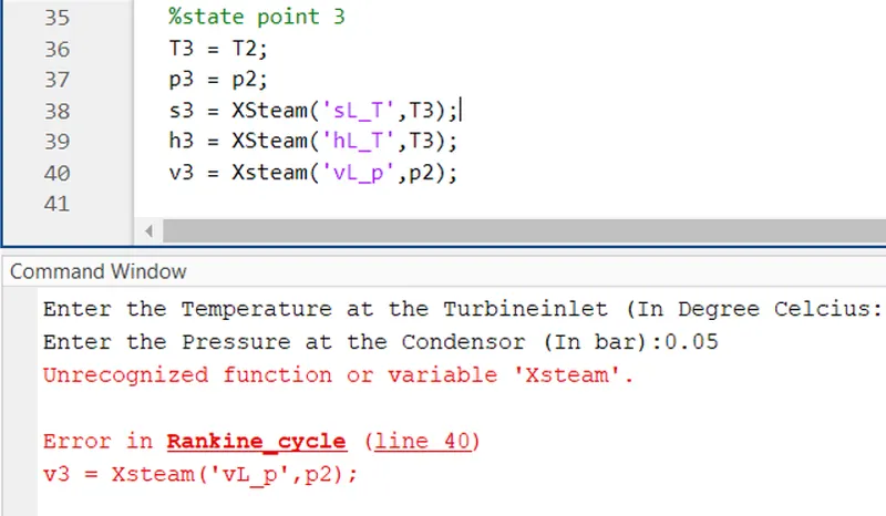
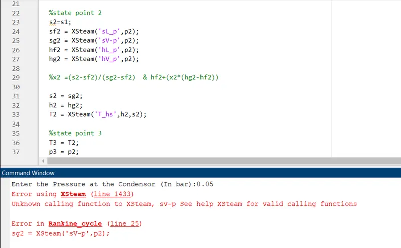
• While programming Found some typos whics is mention on image