Week 4.1 - Genetic Algorithm

OPTIMIZATION -

Optimization is a decision making process, it helps to find best results from set of inputs. Optimization refers to findind the values of inputs in such a way that we get best output values. Best value in mathematical terms which refers in maximizing and minimizing one or more objective functions by varing the input parameters.

GENETIC ALGORITHM -

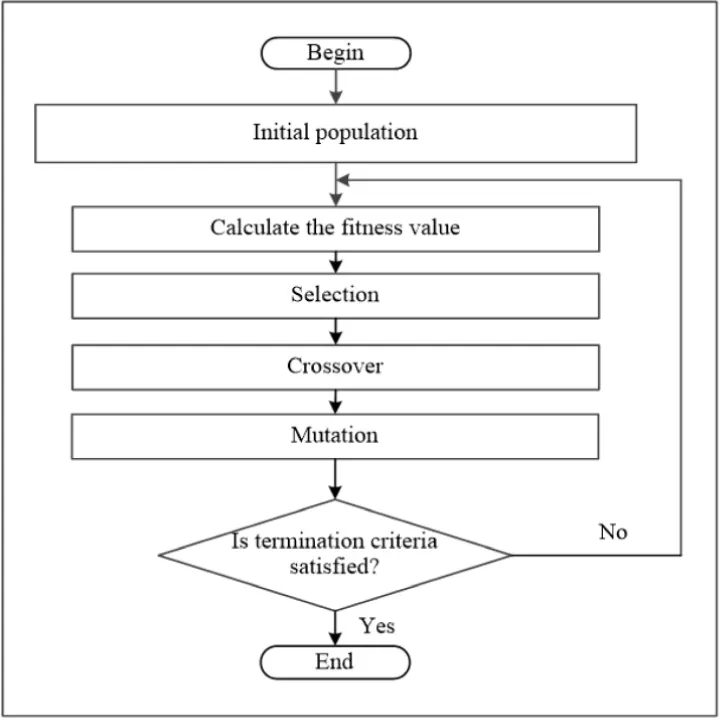
Genetic algorithm is one of the optimization process.Genetic algorithm is a search based optimization technique based on the principles of genetics and natural selection.It is generally used to find optimum and near optimum solutions.

Genetic algorithm is developed by John holland amd his students . In genetic algorithm we have a pool or population of possible solutions to the given problem. These solutions then undergo recombination and mutation and the process is repeated over various generations.

ADVANTAGES OF GENETIC ALGORITHM-

• Genetic algorithm does not require derivative information which is not available to real world problems.
• Optimizes both continious and discrete functions and also multi objective problems.
• Has very good parallel capabilities.
• Provides a list of good solutions and not just single solutions.
• Always gets an answer to the problem which gets better over the time.
• Useful when search space is very large and there are large number of parametrs involved.

LIMITATIONS OF GENETIC ALGORITHM -

• Genetic algorithm are not suited for all problems, especially problems which are simple and for which derivative information is available.
• Fitness value is calculated repeatedly which might be computationally expensive for large problems.
• If not implemented properly the GA may not converge to the optimal solution.
• Being sticastic there is no guarantee on the quality of the solution.

APPLICATIONS OF GENETIC ALGORITHM -

• Genetic algorithm are primarily used in optimization problems of various kinds such as Ecnomics models, neural networks to train neural network, Parallelization , Image processing, vehicle routing problems, scheduling applications and machine learning

AIM -

To write code to calculate Global maxima using Genetic algorithm using MATLAB.

PROCEDURE -

• The stalagmite function is defined separately.This function is later called in to main GA function.
• Now we define x and y values linspace command.
• Then the input vectors are transformed into array [xx yy], so that it can be used to evaluated functions of two variables and plot three dimensional mesh/surface plots.
• Now the values in the different matrixes are created can be put into the function we have created by calling it by this we can get the function of stalagmite function of various values of x and y.
• After obtaining the values of the function at various values we now need to calculate maxima value which can be calculated using ga command, 'ga ' is a in built function in matlab.
• The total time ga needs to be run is defined by using num_cases and with the help of for loop ga is made to run for each iteration and the values are stored in an array.
• Genetic algorithm generally gives minima value but we need to the maxima value hence we can just inverse the stalagmite function by introducing the negative sign.
• The toatal study time is calculated using 'tic' and 'toc' command at the start and end of GA for loop respectively.
• The results are then plotted using surfc and command and plot command.
• GA is made to run for 3 iterations with each iteration having bounded inputs and unbounded inputs and by increasing the population.

The stalagmite function is as follows:

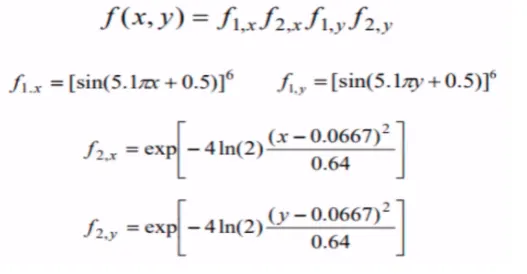
The above stalagmite function is defined as follows :

function [f] = stalagmite(input_value)
x = input_value(1);
y = input_value(2);
f_1 = (sin(5.1*pi*x+0.5))^6;
f_2 = (sin(5.1*pi*y+0.5))^6;
f_3 = exp(-4*log(2)*(x-0.0667)^2/0.64);
f_4 = exp(-4*log(2)*(y-0.0667)^2/0.64);
f = -(f_1*f_2*f_3*f_4);
end

The format for writing genetic algorithm in MATLAB is as follows:

x = ga(fun,nvars,A,b,Aeq,beq,lb,ub,nonlcon,options)

1. x is the local minima point
2. fun is the function to be called
3. nvars indicates no.of variables used.
4. A and b are used to indicate any kind of inequalities that exist in the function.
5. Aeq and Beq also denotes the inequalities.
6. lb = lower bound
7. ub = upper bound
8. nonlcon gives a two vectors representing inequalities and equalities.
9. options are used for additional operations like increasing population size.
10. This is done with the help of ''optimoptions'' .

First iteration:

In the first iteration the behaviour of the algorithm is studied by not defining the limits.The GA doesnot run within a particular searchspace,since we have not defined bounds.

clear all
close all
clc
x = linspace(0,0.6,150);
y = linspace(0,0.6,150);
 
% First Iteration with unbounded limits.

[xx, yy]= meshgrid(x,y);

for i= 1:length(xx)
    for j = 1:length(yy)
        input_value(1)= xx(i,j);
        input_value(2) = yy(i,j);
        f(i,j) = stalagmite(input_value);
    end
end

num_cases = 50;
tic   % Time in count %To find the study time
for i=1:num_cases 
    [inputs,f_opt(i)]= ga(@stalagmite,2);
    x_opt(i)= inputs(1);
    y_opt(i)= inputs(2);
    opt_f(i)= -f_opt(i);
end

study_time = toc 

% Plotting the results
subplot(2,1,1)
hold on 
surfc(xx,yy,f)
shading interp
plot3(x_opt,y_opt,f_opt,'marker','o','markersize',4,'markerfacecolor','r')
title('unbounded inputs')
subplot(2,1,2)
plot(opt_f)
xlabel('Number of iterations')
ylabel('Function Max')
    

Second iteration :

Here the lower and upper bounds are defined so as to know the boundaries within which the global maxima lies. We defining defined were global maxima need to be found out.

clear all
close all
clc
x = linspace(0,0.6,150);
y = linspace(0,0.6,150);

 % second iteration increase in iterations and defined bound 
[xx, yy]= meshgrid(x,y);

for i= 1:length(xx);
    for j = 1:length(yy);
        input_value(1)= xx(i,j);
        input_value(2) = yy(i,j);
        f(i,j) = stalagmite(input_value);
    end
end

num_cases = 100; % GA runs for 100 iterations
tic              % To find the study time
for i=1:num_cases 
    [inputs,f_opt(i)]= ga(@stalagmite,2,[],[],[],[],[0,0],[0.6,0.6]);
    x_opt(i)= inputs(1);
    y_opt(i)= inputs(2);
    opt_f(i) = -f_opt(i); % Here we are doing inverse to find out Maximum value. generally GA finds minimum value
end

study_time = toc  % study time end 

subplot(2,1,1)
hold on 
surfc(xx,yy,f)
shading interp   % To bring smooth curve surface without mesh on the surface 
plot3(x_opt,y_opt,f_opt,'marker','o','markersize',4,'markerfacecolor','r')
title('bounded inputs')
subplot(2,1,2)
plot(opt_f)
xlabel('Number of iterations')
ylabel('Function Max')

Third iteration:

In this code the population size is increased to converge the global maxima.

clear all
close all
clc
x = linspace(0,0.6,150);
y = linspace(0,0.6,150);

 % Third iteration increase in iterations and Population size
[xx, yy]= meshgrid(x,y);

for i= 1:length(xx);
    for j = 1:length(yy);
        input_value(1)= xx(i,j);
        input_value(2) = yy(i,j);
        f(i,j) = stalagmite(input_value);
    end
end

num_cases = 150; % Number of iterations to run is increased
options = optimoptions('ga')
options = optimoptions(options,'populationsize',450)   % Additional operator OPTIONS is used to increase population size
tic       % Time in count 
for i=1:num_cases 
    [inputs,f_opt(i)]= ga(@stalagmite,2,[],[],[],[],[0,0],[0.6,0.6],[],options);
    x_opt(i)= inputs(1);
    y_opt(i)= inputs(2);
    opt_f(i) = -f_opt(i);
end

study_time = toc  %study time ends

subplot(2,1,1)
hold on 
surfc(xx,yy,f)
shading interp
plot3(x_opt,y_opt,f_opt,'marker','o','markersize',4,'markerfacecolor','r')
title('bounded inputs')
subplot(2,1,2)
plot(opt_f)
xlabel('Number of iterations')
ylabel('Function Max')

ERRORS WHILE PROGRAMING :

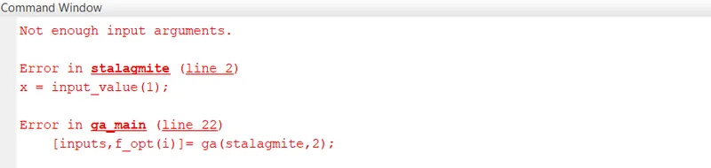
Error calling the staligmite function. where i did not type '@'

RESULTS :

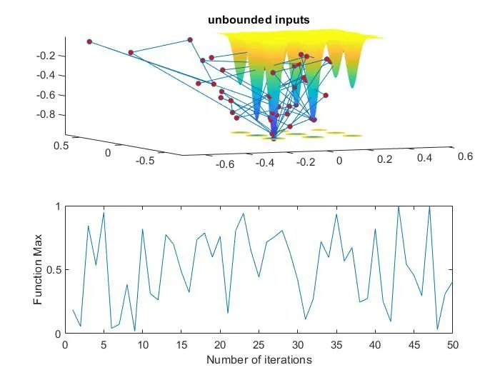
First iteration : (iterations = 50)

In the first iteration it can be seen that since the inputs are boundless GA algorithm has mapped local maxima points outside our stalagmite function.

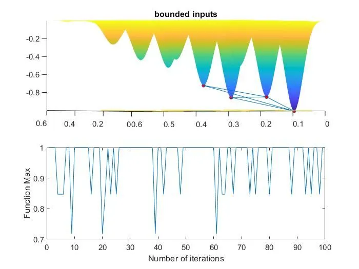
Second iteration (iterations = 100)

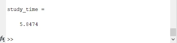
In the second iteration graph is more clear and optimised compared to the first iteration since bounds are defined. The values are within the range.

Third iteration: (iterations = 150 , population size = 450)

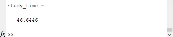
In case we are getting the optimised value of global maxima with accurate range since we increased the number of iterations and population size. since the number of iterations and populoation size increases study time also increases.

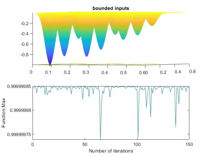
Thus it can be concluded that GA gives more accurate results in case of bounded inputs and by increasing the number of iterations and population size.