Supervised Learning - Prediction Week 3 Challenge

1.Perform Gradient Descent in Python with any loss function

Here i used Mean square error loss function(COST) to find the minimum value.m-curr, b-curr,learning rate, x and Y values are given before defining the function. Here i used Numpy and matplotlib.pyplot libraries to find gradient descent method using Mean square error approach. COST in the script is noting but Mean square error. The best fit line has minimum error. we cannot calculate for each and every line their is a method Minima and maxima.

When we draw graph between M,B and error then we get different error values. for which M and B error value is minimum that is the line we are looking.

MSE = `1/nsum_(i=1)^n(Ya - Yp)^2`

Ya - Y actual , Yp - Y predicted

step 1 - To find Y predicted Yp = M+Bx

step 2 - Substitute Yp in MSE then differentiate the errors to get Tangnets. BY using tangents we move slowly to other point and find the minima. learning rates were give to ensure slow moving rates.

These iterations will go on till we get Minimum error. So i given following Steps in for Loop

import numpy as np
import matplotlib.pyplot as plt

m_curr = b_curr = 0
iterations = 1000
learning_rate = 0.08
x=np.array([1, 2, 3, 4, 5])
y=np.array([5, 7, 9, 11, 13])
n =len(x)

COST = []
B = []
M = []
Z = []
for i in range(iterations):
    y_predicted = m_curr * x + b_curr
    cost = (1 / n) * sum([val ** 2 for val in (y - y_predicted)])
    md = -(2 / n) * sum(x * (y - y_predicted))
    bd = -(2 / n) * sum((y - y_predicted))
    m_curr = m_curr - learning_rate * md
    b_curr = b_curr - learning_rate * bd
    print("m {}, b {}, cost {}, iteration {}".format(m_curr, b_curr, cost, i))
    COST.append(cost)
    M.append(m_curr)
    B.append(b_curr)
    Z.append(i)
plt.scatter(M, COST)
plt.show()
plt.scatter(B, COST)
plt.show()
plt.scatter(Z, COST)
plt.show()

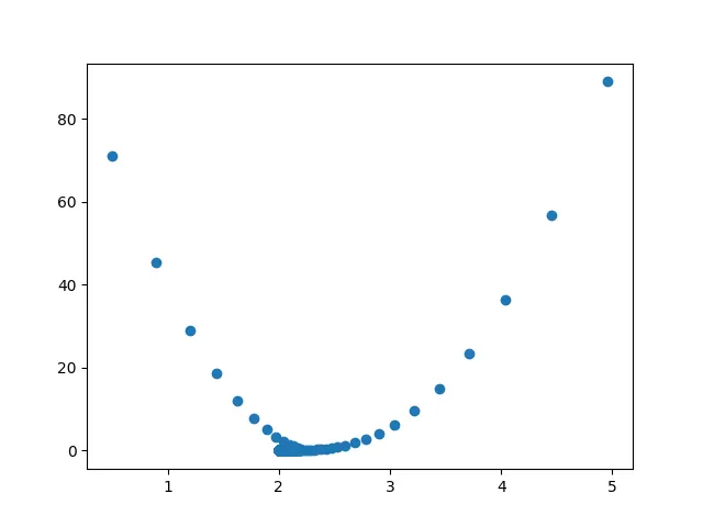
Graph Versus M and COST

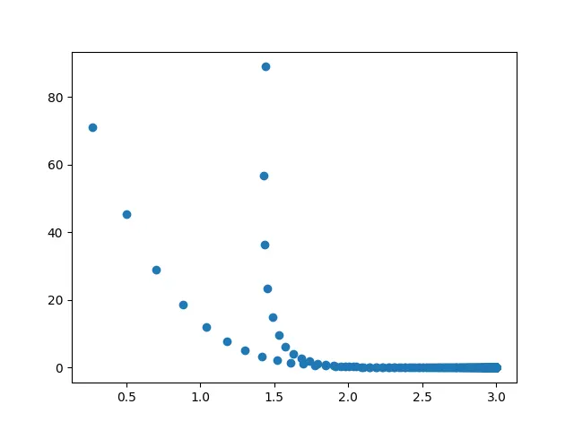
Graph Versus B and COST

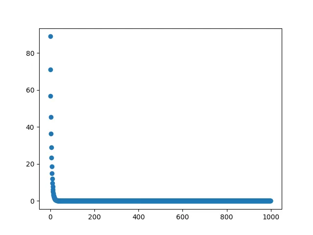
Graph Versus iterations and COST

2.Difference between L1 & L2 Gradient descent method

ans - L1 - Mean absolute error

L2 - Mean square error

The advantage of the MAE is that its adavantage directly covers the MSE diadvantage. In MAE all the errors will be weighted on the same linear scale. The disadvantage of MAE is large errors coming from outliers end up being weighted the exact same as lower errors

The advantage with MSE is great ensuring that our trained model has no outlier predictions with huge errors since MSE puts larger weight on these errors due to squaring part of the function. The diadavantage with MSE is the squaring part of the function magnifies the error

3.What are the different loss functions for regression

ans - Loss function is nothing but calculating error. their are 3 different types of errors

• Root mean square error
• Mean square error
• Mean absolute error

4.What is the importance of learning rate

ans - In the process of finding best linear fit . As we find Y(predicted)[error] from one of the loss function , deferentiation of error gives tangent , but we want tangent to move slowly then learning rate comes into picture. The importance of linear rate is it allows the tangents to move slowly. most cases learning rate is 0.001 .

5.How to evaluate linear regression

ans - Coefficient of determination (R^2). If the R^2 is close to one then our prediction what we are making are with good accuracy.R^2 value going down means prediction is wrong completely. makesure R^2 close to one. R^2 is a measure of evaluating the best fit curve.

6.What is the difference between multiple and adjusted coefficient of determination

ans - Adjusted coefficient of determination is modified version of coefficient of determination(R^2). In adjusted coefficient of determination will increase only if a new data point improves the regression more than you expected. adjusted coefficient of determination does not include all data points it is always lower than coefficient of determination(R^2).

The multiple coefficient of determination measures the portion of variation in the dependent variable that can be predicted from independent variables

multiple coefficient of determination =

sum of squares of determination / total sum of squares