Week 3.5 - Deriving 4th order approximation of a 2nd order derivative using Taylor Table method
PROJECT-
To calculate the 2nd order derivative of the analytic function `exp(x)*cos(x)` and compare
with the three numerical approximation that given using matlab.
- Central difference
- Skewed right sided difference
- skewed left sided difference
THEORY-
Taylor table is a type of table which cointains the data of all the taylor series expansion of a function
that can beused to calculate th eanalytical value of the higher order derivative and use to help
calculate the numerical discretization . The best thing about the taable is the more term it have
the more acuracy we will get .
OBJECTIVE-
Derive the given 4th order approximatiomnthe of the 2nd order derivative.
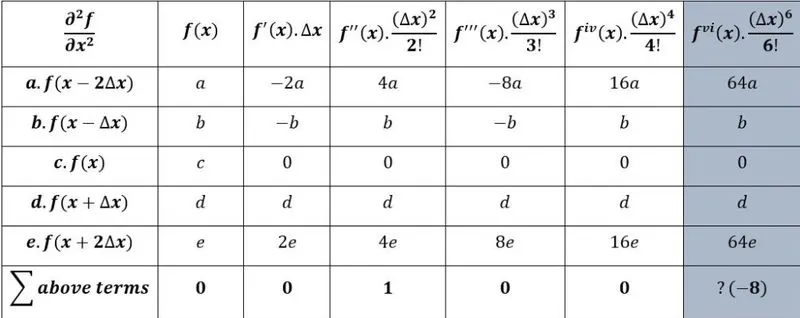
CENTRAL DIFFERENCE SCHEME-
`(del^2f)/dx^2 = afunderset(i-2)+bf underset(i-1)+cfunderset(i)+dfunderset(i-1)+efunderset(i+2)`
`a{funderset(i-2)`}=`a{funderseti-(2Deltax)/(1!)f'underseti+(2Deltax)^2/(2!)f''underseti+(2Deltax)^3/(3!)f'''underseti+(2deltax)^4/(4!)f''''underseti}`}
`{funderset(i-1)`}=`b{funderseti-(Deltax)/(1!)f'underseti+(Deltax)^2/(2!)f''underseti-(Deltax)^3/(3!)f'''underseti+(Deltax)^4/(4!)f''''underseti``
`cfunderseti`=`cfunderseti`
`d{funderseti`}=`d{funderseti+(Deltax)/(1!)+(Deltax^2)/(2!)f''underseti+(Deltax^3)/(3!)f'''underseti+(Deltax^4)/(4!)f''''underseti`}
`e{funderset(i+2)`}=`e{funderseti+(2Deltax)/(1!)f''underseti+(2Deltax^2)/(2!)f''underseti+(2Deltax^3)/(3!)f'''underseti+(2Deltax^4)/(4!)f''''underseti+`
TAYLOR TABLE FOR CDS-
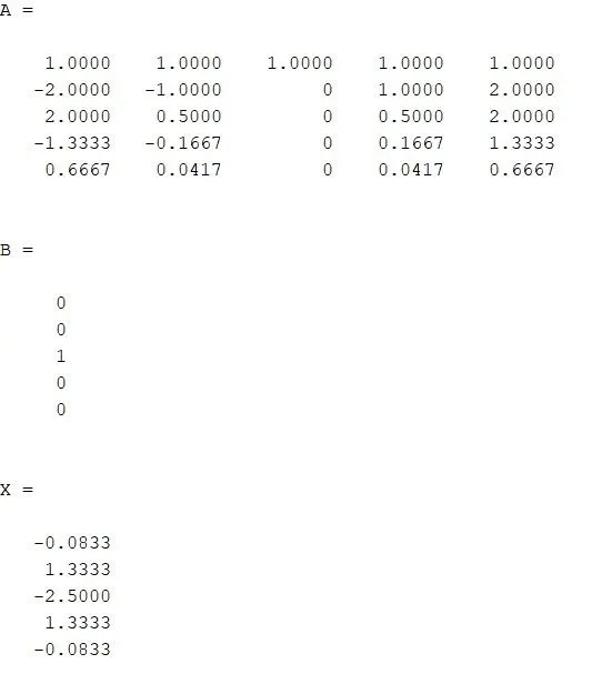
MATLAB CODE TO FIND THE VALUE OF (a,b,c,d,e)
clear all
close all
clc

% A
 A = [1 1 1 1 1;-2 -1 0 1 2;2 1/2 0 1/2 2;-4/3 -1/6 0 1/6 4/3;2/3 1/24 0 1/24 2/3]
% B
 B = [0;0;1;0;0]
% X
 X = linsolve(A,B)
RESULT-
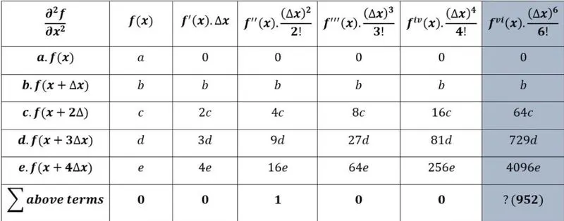
SKEWED RIGHT SIDED DIFFERENCE-
`(del^2f)/dx^2 = afunderset(i)+bf underset(i+1)+cfunderset(i+2)+dfunderset(i+3)+efunderset(i+4)`
`afunderseti``= afunderseti`
`b{funderset(i+1)`}=`b{funderseti+(Deltax)/(1!)f'underseti+(Deltax^2)/(2!)f''underseti+(Deltax^3)/(3!)f'''underseti+(Deltax^4)/(4!)f''''underseti+`}
`c{funderset(i+2)`}=`c{funderseti+(2Deltax)/(1!)f'underseti+(2Deltax^2)/(2!)f''underseti+(2Deltax^3)/(3!)f'''underseti+(2Deltax^4)/(4!)f''''underseti+`}
`d{funderset(i+3)`}=`d{funderseti+(3Deltax)/(1!)f'underseti+(3Deltax^2)/(2!)f''underseti+(3Deltax^3)/(3!)f'''underseti+(3Deltax^4)/(4!)f''''underseti+`}
`e{funderset(i+4)`}=`e{funderseti+(4Deltax)/(1!)f'underseti+(4Deltax^2)/(2!)f''underseti+(4Deltax^3)/(3!)f'''underseti+(4Deltax^4)/(4!)f''''underseti+``
TAYLOR TABLE FOR SKEWED RIGHT SIDED DIFFERENCE-
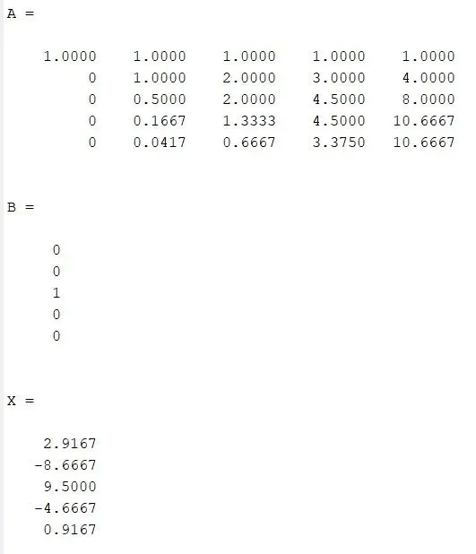
MATLAB CODE TO FIND THE VALUE OF (a,b,c,d,e)
clear all
close all
clc
% A
 A = [1 1 1 1 1;0 1 2 3 4;0 1/2 2 9/2 8;0 1/6 4/3 9/2 32/3;0 1/24 2/3 27/8 32/3]
% B
 B = [0;0;1;0;0]
% X
 X = linsolve(A,B)
RESULT-
SKEWED LEFT SIDED DIFFERENCE-
`(del^2f)/dx^2 = afunderset(i)+bf underset(i-1)+cfunderset(i-2)+dfunderset(i-3)+efunderset(i-4)`
`afunderseti``= afunderseti`
`b{funderset(i-1)`}=`b{funderseti-(Deltax)/(1!)f'underseti+(Deltax^2)/(2!)f''underseti-(Deltax^3)/(3!)f'''underseti+(Deltax^4)/(4!)f''''underseti+``
`c{funderset(i-2)`}=`c{funderseti-(2Deltax)/(1!)f'underseti+(2Deltax^2)/(2!)f''underseti-(2Deltax^3)/(3!)f'''underseti+(2Deltax^4)/(4!)f''''underseti`}
`d{funderset(i-3)`}=`d{funderseti-(3Deltax)/(1!)f'underseti+(3Deltax^2)/(2!)f''underseti-(3Deltax^3)/(3!)f'''underseti+(3Deltax^4)/(4!)f''''underseti+`}
`e{funderset(i-4)`}=`e{funderseti-(4Deltax)/(1!)f'underseti+(4Deltax^2)/(2!)f''underseti-(4Deltax^3)/(3!)f'''underseti+(4Deltax^4)/(4!)f''''underseti+`}
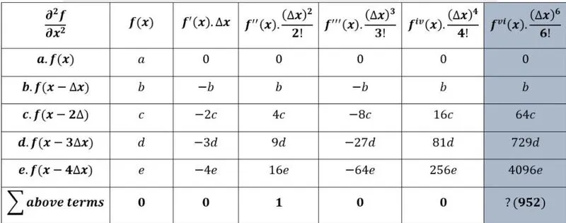
TAYLOR TABLE FOR SKEWED LEFT DIFFERENCE-
MATLAB CODE TO FIND THE VALUE OF (a,b,c,d,e)
clear all
close all
clc
% A
 A = [1 1 1 1 1;0 1 2 3 4;0 1/2 2 9/2 8;0 1/6 4/3 9/2 32/3;0 1/24 2/3 27/8 32/3]
% B
 B = [0;0;1;0;0]
% X
 X = linsolve(A,B)
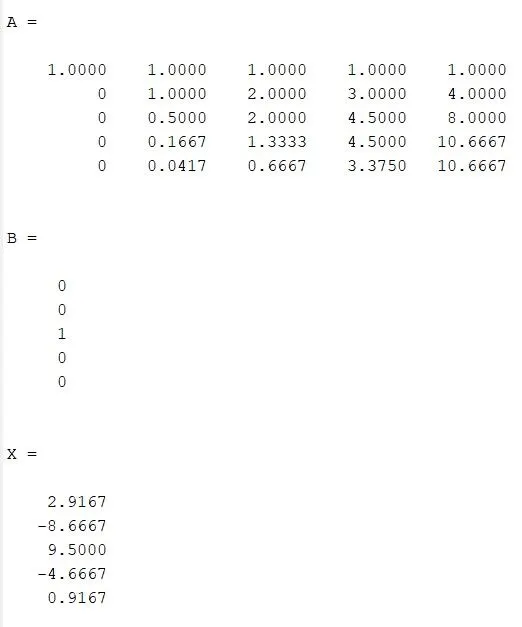
RESULT-
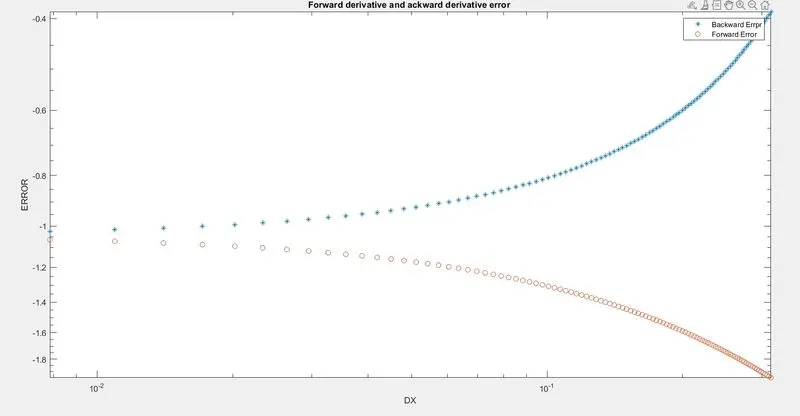
MATLAB CODE - THE ERROR AT DIFFERENT VALUE FOR FORWARD DERIVATIVE AND BACKWAARD DERIVATIVE COMPARED WITH ANALYTICAL DERIVATIVE
clear all
close all
clc

% Analytical function f' = exp(x)*cos(x)
%f'' = -2exp(x)*sin(x)
x = pi/3;

%Range of the matrix of dx
dx = linspace(pi/10,pi/400,100);
Analytical_function = exp(x)*cos(x);
Analytical_derivative = -2*exp(x)*sin(x);

for i = 1:length(dx)
    b_derivative(i) =(exp(x)*cos(x)-exp(x-dx(i))*cos(x-dx(i)))/dx(i)
    f_derivative(i) =(exp(x+dx(i))*cos(x+dx(i))-exp(x)*cos(x))/dx(i)
    error_b(i)= abs(b_derivative(i)-Analytical_derivative)
    error_f(i)= abs(f_derivative(i)-Analytical_derivative)
end

%Ploting(using loglog comand)
loglog(dx,b_derivative,'*')
hold on
loglog(dx,f_derivative,'o')
hold off
xlabel('DX')
ylabel('ERROR')
legend('Backward Errpr','Forward Error')
title('Forward derivative and ackward derivative error ')
RESULT-
FUNCTION CODE-
-ABSOLUTE ERROR BETWEEN 2ND ORDER DERIVATIVE AND CENTRAL DIFFERENCE
function error_central_differnce = central_difference(x,dx)
% Function
% f' = exp(x)*cos(x)

%second order derivative of the function
second_order_derivative =-2*exp(x)*sin(x)

%skewed right difference value
central_difference=((-0.0833)*(exp(x-(2*dx))*cos(x-(2*dx)))+(1.3333)*(exp(x-(1*dx))*cos(x-(1*dx)))+(-2.50000)*(exp(x)*cos(x))+(1.3333)*(exp(x+(1*dx))*cos(x+(1*dx)))+(-0.08333)*(exp(x+(2*dx))*cos(x+(2*dx))))/(dx^2)

%error
error_central_differnce = abs(second_order_derivative-central_difference)
end
-ABSOLUTE ERROR BETWEEN 2nd ORDER DERIVATIVE AND SKEWED RIGH DIFFERENCE
function error_skewed_DR = skewed_difference_right(x,dx)
% Function
% f' = exp(x)*cos(x)

%second order derivative of the function
second_order_derivative =-2*exp(x)*sin(x)

%skewed right difference value
skewed_difference_right=(((2.9166)*(exp(x))*(cos(x)))+((-8.666)*(exp(x+(1*dx)))*cos(x+(1*dx)))*((9.5)*(exp(x+(2*dx)))*cos(x+(2*dx)))+((-4.666)*(exp(x+(3*dx)))*cos(x+(3*dx)))+((0.9166)*(exp(x+(4*dx)))*cos(x+(4*dx))))/(dx^2);

%error
error_skewed_DR = abs(second_order_derivative-skewed_difference_right)
end
-ABSOLUTE ERROR BETWEEN 2nd ORDER DERIVATIVE AND SKEWED LEFT DIFFERENCE
function error_skewed_DL = skewed_difference_left(x,dx)
% Function
% f' = exp(x)*cos(x)
%second order derivative of the function
second_order_derivative =-2*exp(x)*sin(x)
%skewed right difference value
skewed_difference_left=(((2.9166)*(exp(x))*(cos(x)))+((-8.666)*(exp(x-(1*dx)))*cos(x-(1*dx)))*((9.5)*(exp(x-(2*dx)))*cos(x-(2*dx)))+((-4.666)*(exp(x-(3*dx)))*cos(x-(3*dx)))+((0.9166)*(exp(x-(4*dx)))*cos(x-(4*dx))))/(dx^2);
%error
error_skewed_DL = abs(second_order_derivative-skewed_difference_left)
endMAIN PROGRAM-
clear all
close all
clc

% Function is f(x)=sin(x)/x^3
x = pi/3;

% Range of the matrix of dx
dx = linspace(pi/10,pi/4000,200)

for i= 1:length(dx)
    skewed_difference_right_value(i)=skewed_difference_right(x,dx(i))
    skewed_difference_left_value(i)=skewed_difference_left(x,dx(i))
    central_difference_value(i)=central_difference(x,dx(i))
end

%Ploting
loglog(dx,skewed_difference_right_value)
hold on
loglog(dx,skewed_difference_left_value)
hold on
loglog(dx,central_difference_value)
hold off
xlabel('Dx')
ylabel('(ERROR)')
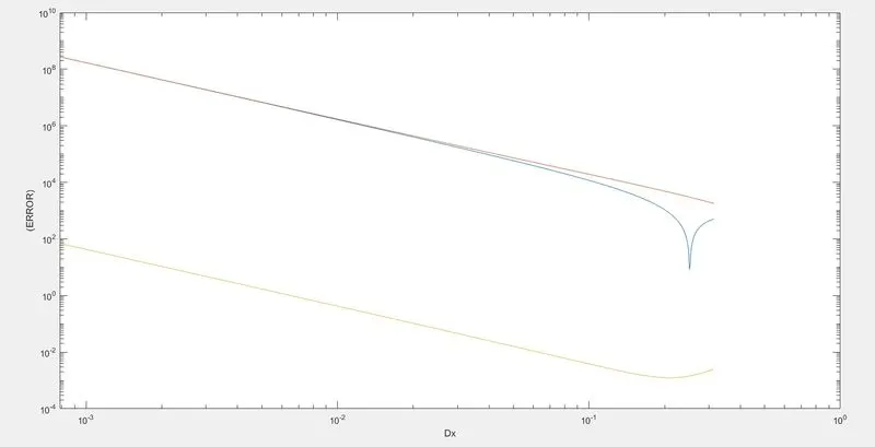
RESULT-
CONCLUSION-
If we apply approximation at boundaries ,in central difference scheme we are too close to the
result beacuse it calculate both forwade and backward value.