Challenge

Week 4.1 - Genetic Algorithm

SSuraj Mullla8 Jan 2022

AIM:-To write a code in MATLAB to optimise the stalagmite function and find the global maxima of the function.

GENETIC ALGORITHM

The genetic algorithm is a method for solving both constrained and unconstrained optimization problems that is based on natural selection it is same the process drives biological evolution.

natural selection is the biological term derived by the charles darwin which occurs during the evolution of the organism.

In such a way, genetic algorithm modifies a population of individual solutions again and again so that at each step, the genetic algorithm selects individuals at random from the current population to be parents and uses them to produce the children for the next generation. Over successive generations, the population "evolves" toward an optimal solution.

we can apply the genetic algorithm to solve a variety of optimization problems that are not well suited for standard optimization algorithms, including problems in which the objective function is discontinuous, nondifferentiable, stochastic, or highly nonlinear. The genetic algorithm can address problems of mixed integer programming, where some components are restricted to be integer-valued.

The genetic algorithm uses three main types of rules at each step to create the next generation from the current population:

Selection rules select the individuals, called parents, that contribute to the population at the next generation.
Crossover rules combine two parents to form children for the next generation.
Mutation(sudden change) rules apply random changes to individual parents to form children.

syntax of ga

x = ga(fun,nvars,A,b) finds a local minimum x to fun, subject to the linear inequalities A*x ≤ b. ga evaluates the matrix product A*x as if x is transposed (A*x')

x= ga(fun,nvars,A,b,Aeq,beq) finds a local minimum x to fun, subject to the linear equalities Aeq*x = beq and A*x ≤ b. (Set A=[] and b=[] if no linear inequalities exist.) ga evaluates the matrix product Aeq*x as if x is transposed (Aeq*x')

x= ga(fun,nvars,A,b,Aeq,beq,lb,ub) defines a set of lower and upper bounds on the design variables, x, so that a solution is found in the range lb ≤ x ≤ ub. Set Aeq=[] and beq=[] if no linear equalities exist.

x = ga(fun,nvars,A,b,Aeq,beq,lb,ub,nonlcon) subjects the minimization to the constraints defined in nonlcon. The function nonlcon accepts x and returns vectors C and Ceq, representing the nonlinear inequalities and equalities respectively. ga minimizes the fun such that C(x) ≤ 0 and Ceq(x) = 0. (Set lb=[] and ub=[] if no bounds exist.

x = ga(fun,nvars,A,b,Aeq,beq,lb,ub,nonlcon,option) minimizes with the default optimization parameters replaced by values in options. (Set nonlcon=[] if no nonlinear constraints exist.) Create options using optimoption.
x = ga(fun,nvars,A,b,Aeq,beq,lb,ub,nonlcon,intcon) or x = ga(fun,nvars,A,b,Aeq,beq,lb,ub,nonlcon,intcon,option) requires that the variables listed in intcon take intege

A code in MATLAB to optimise the stalagmite function and find the global maxima of the function.

step-1:-we have to creat stalagmite function

A stalagmite function generally refers to the function with which we are generating values over a stalagmite kind of surface for finding out the local and global maxima and minima of that particular given function.

using equation:

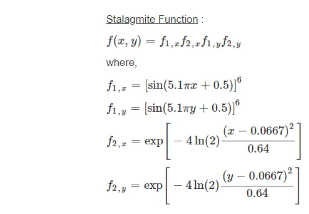
stalagmite function:-

% creating a stalagmite function
function [f] =stalagmite(input_vector)
x=input_vector(1);
y=input_vector(2);

t1=(sin((5.1*pi*x)+0.5))^6;
t2=(sin((5.1*pi*y)+0.5))^6;
t3=exp(-4*log(2)*((x-0.0667)^2)/0.64);
t4=exp(-4*log(2)*((y-0.0667)^2)/0.64);

f=-(t1*t2*t3*t4);
end

step:-2

write a code to determine global maxima

start with clear all ,close all and clc.
introduce a inputs
creat 2d mesh using meshgrid [X,Y] = meshgrid(x,y) returns 2-D grid coordinates based on the coordinates contained in vectors x and y. X is a matrix where each row is a copy of x, and Y is a matrix where each column is a copy of y. The grid represented by the coordinates X and Y has length(y) rows and length(x) columns.
evaluate the stalagmite function
creat for loop and define the i and j value
use a tic and toc commad .A tic works with the toc function to measure elapsed time. The tic function records the current time, and the toc function uses the recorded value to calculate the elapsed time.Passing this value is useful when there are multiple calls to tic to time different parts of the same code.
use ga commad
A surfc( X , Y , Z ) creates a three-dimensional surface plot with a contour plot underneath
plot3( X , Y , Z ) plots coordinates in 3-D space.
use shading interp to remove grid so the graph will look more smooth.
plot the graph
also find the global maxima

code :-

clear all
close all
clc
%inputs
x=linspace(0,0.6,150);
y=linspace(0,0.6,150);
num_case=50;
%creating a 2d mesh
[xx yy] =meshgrid(x,y);

%evaluting stalagmite function
for i=1:length(xx)
for j=1:length(yy)
input_vector(1)=xx(i,j);
input_vector(2)=yy(i,j);
f(i,j)=stalagmite(input_vector);
end
end
%study 1
tic
for i=1:num_case
[inputs,fopt(i)]=ga(@stalagmite,2);
xopt(i)=inputs(1);
yopt(i)=inputs(2);
end
study1_time=toc

figure(1)

subplot(2,1,1)
hold on
surfc(xx,yy,-f)
shading interp
xlabel('x-axis')
ylabel('y-axis')
title('statistical behaviour with unbound inputs')
plot3(xopt,yopt,-fopt,'marker','o','markersize',5,'markerfacecolor','r')
subplot(2,1,2)
plot(-fopt)
xlabel('no. of iteration')
ylabel('function maximum')

study2_time=toc

figure(2)

subplot(2,1,1)
hold on
surfc(xx,yy,-f)
shading interp
xlabel('x-axis')
ylabel('y-axis')
title('statistical behaviour with unpper and lower bounds')
plot3(xopt,yopt,-fopt,'marker','o','markersize',5,'markerfacecolor','r')
subplot(2,1,2)
plot(-fopt)
xlabel('no. of iteration')
ylabel('function maximum')
%study3 : statistical behaviour with increasing iteration of GA
options =optimoptions('ga');
options =optimoptions(options,'populationSize',300);
tic
for i=1:num_case
[inputs,fopt(i)] =ga(@stalagmite,2,[],[],[],[],[0;0],[1;1],[],[],options);
xopt(i) =inputs(1);
yopt(i)=inputs(2);
end
study3_time=toc

figure(3)
subplot(2,1,1)
hold on
surfc(xx,yy,-f)
shading interp
xlabel('X-axis')
ylabel('y-axis')
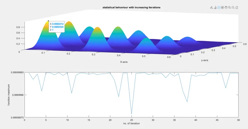
title('statistical behaviour with increasing iterations')
plot3(xopt,yopt,-fopt,'marker','o','markersize',5,'markerfacecolor','r')
subplot(2,1,2)
plot(-fopt)
xlabel('no. of iteration')
ylabel('function maximum')
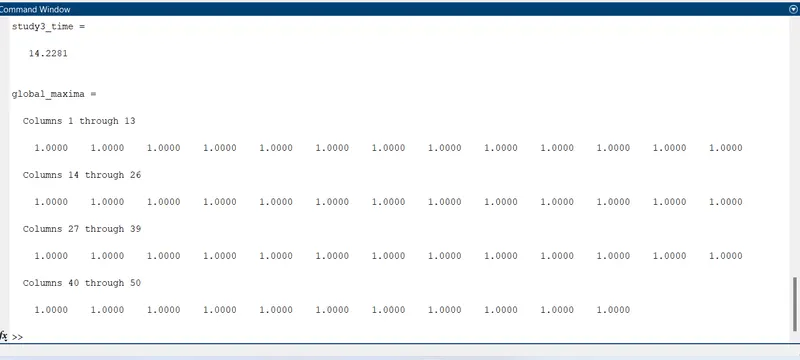
global_maxima=-fopt

Results :-

output graphs

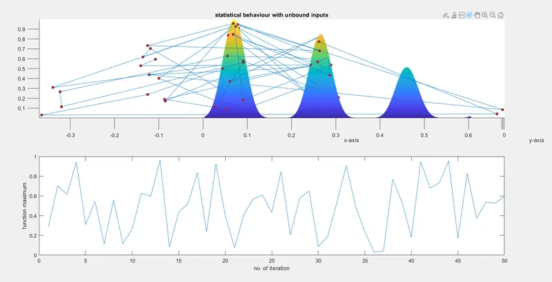
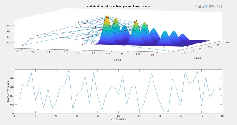
values of (x,y,z) in figure of incresing iteration is shown

output of global maxima:-

Week 4.1 - Genetic Algorithm

Ship work like this
in your own course.

Talk to a career counsellor

Ship work like thisin your own course.

Talk to a career counsellor

Ship work like this
in your own course.