Project 1 - Parsing NASA thermodynamic data
Aim : To write a code in matlab to parse the NASA thermodynamic data and then calaculate the thermodynamic properties of various gas species.
File parsing refers to how information can be read from a particular text file and how that information can be used in program. Parsing a file means reading in a data stream and building a memory model of the content of that data. This aims at facilitating perfoming some kind of transformation on the data. Parsing splits a file or other input into pieces of data that can be easily stored or manipulated.
step 1 -start with clearing back data using clear all, close all ,clc .
step 2-acces the desire file using fopen.
step 3 -read the data using fgetl command.
step 4- get the required lines and skip the lines which are not useful for calculation using for loops.
step 5-use strsplit to split the temperature data.
step 6-use str2num to convert the string into the number.
step 7-strfind to find the string.
step 8-add the gas constant.
step 9-extract the coefficients.
step-10 -using formulas given above calculate and plot the data
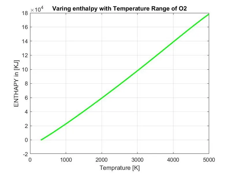
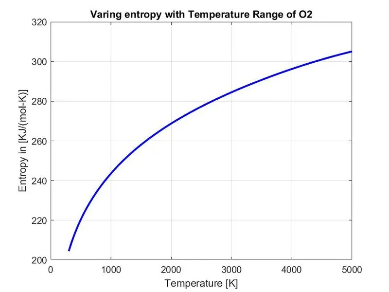
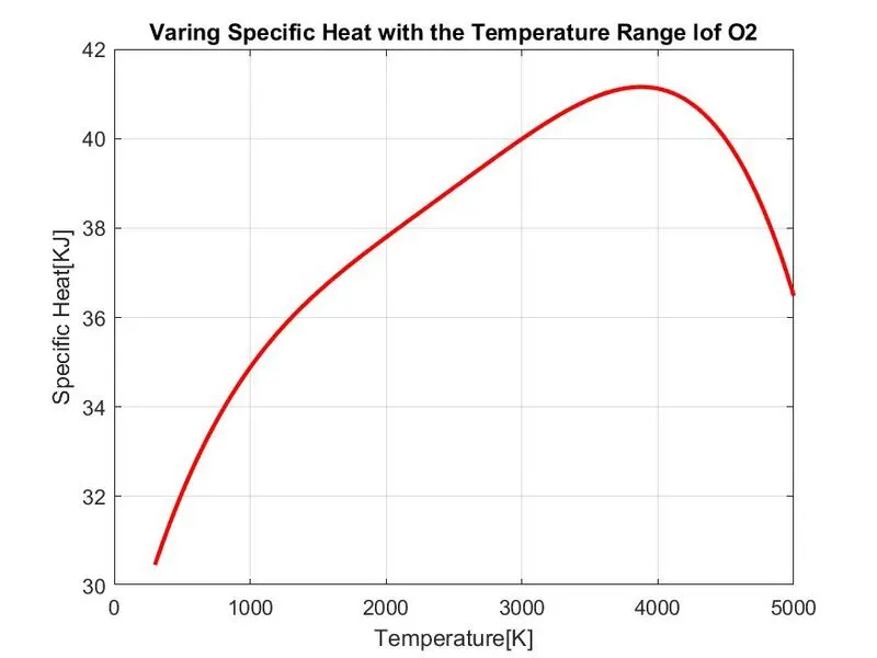
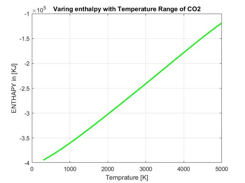
step-10-plot the graphs of enthalpy,entropy and specific heat.
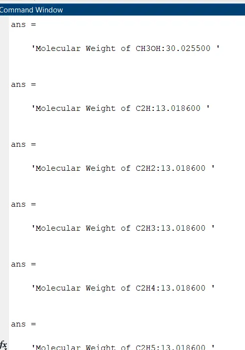
step11-calculate the molecular weight.
code:
clear all
close all
clc
%getting the data file
f1=fopen('THERMO.dat','r');
fgetl(f1)
%reading the header information
A=fgetl(f1);
A=strsplit(A,' ') ;
g1obal_low_temp=str2num(A{2});
g1oba1_mid_temp=str2num(A{3}) ;
g1oba1_h1gh_temp=str2num(A{4}) ;
%skipping next three lines
for i=1:3
fgetl(f1);
end
%reading the species
for i=1:53
header=fgetl(f1);
x=strsplit(header,' ');
species_name=(x{1});
z=length(x);
local_low_temp=str2num(x{z-3});
local_high_temp=str2num(x{z-2});
local_mid_temp=str2num(x{z-1});
t1=local_low_temp;
t2=local_mid_temp;
t3=local_high_temp;
%getting first line coeffecients (a1-a5)
line_1=fgetl(f1);
a=strfind(line_1,'E');
a1=str2num(line_1(1:a(1)+3));
a2=str2num(line_1(a(1)+4:a(2)+3));
a3=str2num(line_1(a(2)+4:a(3)+3));
a4=str2num(line_1(a(3)+4:a(4)+3));
a5=str2num(line_1(a(4)+4:a(5)+3));
%getting second line coeffzceints (a6-all)
line_2=fgetl(f1);
a_1=strfind(line_2,'E');
a6=str2num(line_2(1:a_1(1)+3));
a7=str2num(line_2(a_1(1)+4:a_1(2)+3));
a8=str2num(line_2(a_1(2)+4:a_1(3)+3));
a9=str2num(line_2(a_1(3)+4:a_1(4)+3));
a10=str2num(line_2(a_1(4)+4:a_1(5)+3));
%getting third line coeffecRints(a10-al4)
line_3=fgetl(f1);
a_2=strfind(line_1,'E' );
a11=str2double(line_3(1:a_2(1)+3));
a12=str2double(line_3(a_2(1)+4:a_1(2)+3));
a13=str2double(line_3(a_2(2)+4:a_1(3)+3));
a14=str2double(line_3(a_2(3)+4:a_1(4)+3));
%creating folder
%mkdir([ 'C:\Users\HP',species_name]
T=linspace(t1,t3,1000);
R=8.314;
% to get array of specific heat, enthalpy and entropy
for k=1:length(T)
% to compare the species temperature to assign the coeffeceints
%a1-a7 (high temperature coef eceints), a8-a14(low temperature coeffecients)
if T(k)>t2
%high temperature coeffeceints.
cp=(a1+a2.*T+a3.*T.^2+a4.*T.^3+a5.*T.^4)*R;
H=(a1+(a2.*T)/2+(a3.*T.^2)/3+(a4.*T.^3)/4+(a5.*T.^4)/5+(a6./T))*R.*T;
S=a1.*log(T)+a2.*T+(a3.*T.^2)/2+(a4.*T.^3)/3+(a5.*T.^4)/4+a7;
else
%low temperature coeffecients
cp=(a8+a9.*T+a10.*T.^2+a11.*T.^3+a12.*T.^4)*R;
H=(a8+(a9.*T)/2+ (a10.*T.^2)/3+(a11.*T.^3)/4+(a12.*T.^4)/5+(a13./T))*R.*T;
S=a8.*log(T)+a9.*T+(a10.*T.^2)/2+(a11.*T.^3)/3+(a12.*T.^4)/4+a14;
end
end
%plotting the graphs
figure(1);
plot(T,cp,'linewidth',2,'color','r');
grid on ;
title(sprintf('Varing enthalpy with Temperature Range of %s',species_name));
xlabel('Temperature[K]');
ylabel( 'Specific Heat [KJ]') ;
figure(2);
plot(T,H,'linewidth',2,'color','g');
grid on ;
title(sprintf('Varing enthalpy with Temperature Range of %s',species_name));
xlabel(''Temperature[K]');
ylabel('Enthalpy[KJ]');
figure(3);
plot(T,S,'linewidth',2,'color','b');
grid on ;
title(sprintf('Varing enthalpy with Temperature Range of %s',species_name));
xlabel('Temperature[K]');
ylabel('Entropy[KJ]');
%changing the directory and saving the file
saving=(['C:\Users\HP\',species_name]);
saveas(1,'specific heat','jpg');
saveas(2,'enthalpy','jpg');
saveas(3,'entropy','jpg' );
%molecular_masscalculation
elements=['H','C','O','N', 'A'];
atomic_weight=[1.0079 12.0107 15.999 14.0067 39.948];
mol_mass=0;
for l=1:length(species_name)
for m=1:length(atomic_weight)
if strcmp(species_name(l),elements(m))
mol_mass=mol_mass+atomic_weight(m);
position = m;
end
end
n=str2double(species_name(1));
if n>1
mol_mass= mol_mass+atomic_weight(position)*(n-1);
end
end
sprintf('Molecular Weight of %s:%f ',species_name,mol_mass)
end
fclose(f1)
output :
Screenshot of the window where all the folders are saved

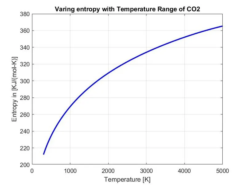
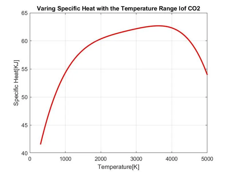
Plots for o2, N2 and Co2 species:
02
N2
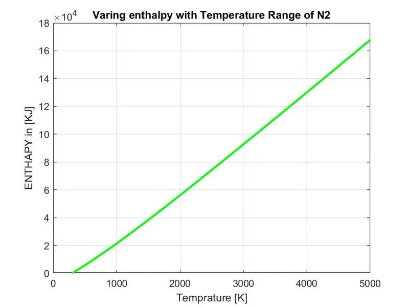
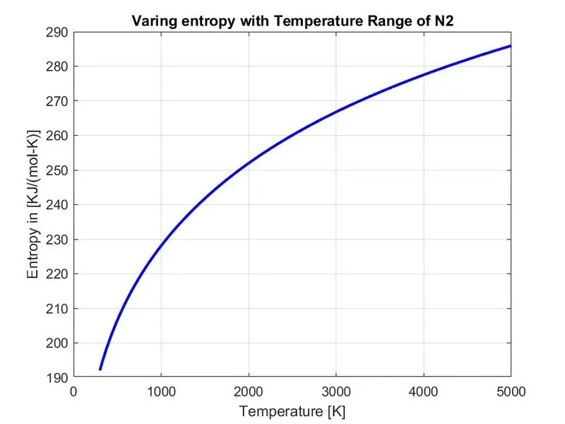
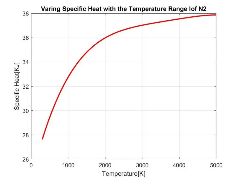
CO2
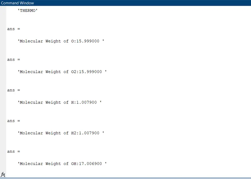
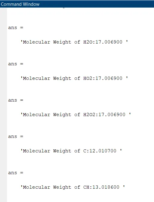
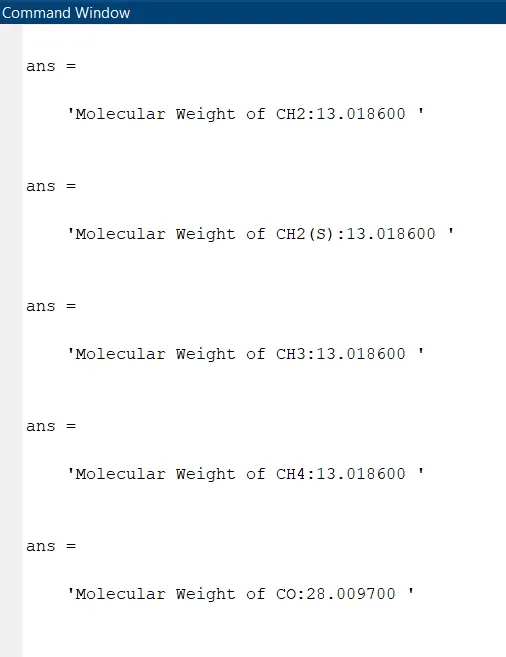
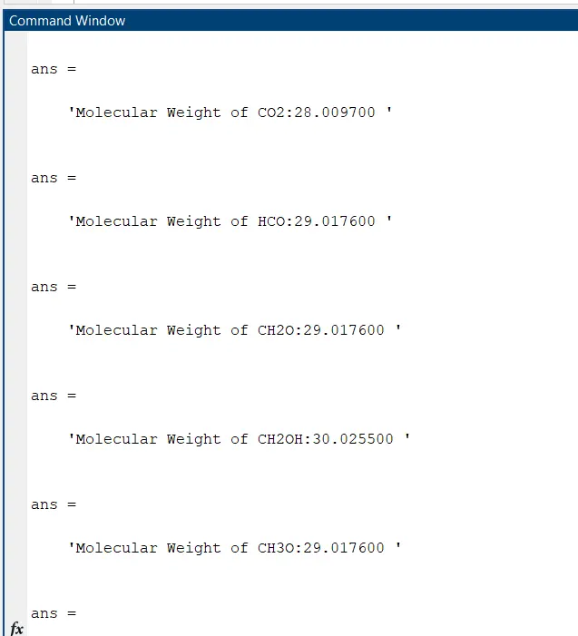
molecular weight of each species in the command window