Project 2 - Rankine cycle Simulator

Aim- Create a Rankine Cycle Simulator using OCTAVE/MATLAB and calculate the state points of the Rankine Cycle based on user input.

abstract:

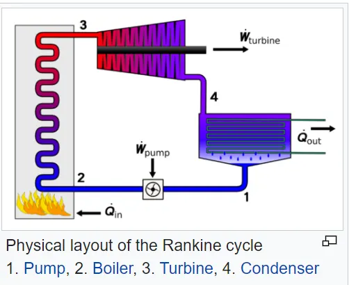
• The Rankine cycle closely describes the process by which steam engines commonly found in thermal power generation plant harness the thermal energy of a fuel or other heat source to generate electricity.

There are four processes in the Rankine cycle.

The states are identified by numbers in the T-s diagram

• Process 1–2: The working fluid is pumped from low to high pressure. As the fluid is a liquid at this stage, the pump requires little input energy. Process 1-2 is isentropic compression.
• Process 2–3: The high-pressure liquid enters a boiler, where it is heated at constant pressure by an external heat source to become a dry saturated vapour. The input energy required can be easily calculated graphically, using an enthalpy-entropy chart , or numerically, using steam tabelor software. Process 2-3 is constant pressure heat addition in boiler.
• Process 3–4: The dry saturated vapour expands through a turbine, generating power. This decreases the temperature and pressure of the vapour, and some condensation may occur. The output in this process can be easily calculated using the chart or tables noted above. Process 3-4 is isentropic expansion.
• Process 4–1: The wet vapour then enters a condenser, where it is condensed at a constant pressure to become a saturated liquid. Process 4-1 is constant pressure heat rejection in condenser.

steps to perform experiment:

• start code using clear all, close all, clc.
• using fprintf print the statements.
• insert user based inputs using input which are required in calculation.
• get the required data from the xsteam by saving the file in same directory .
• seprate the states of process as state point 1,state point 2,state point 3 and state point 4.
• calculate Work done, heat SsC and efficiency calculation using formulas.
• plot the T-s and H-s graph using plot command and add the colour and title using 'color' and title command.

Code :

clear all
close all
clc

fprintf('SIMULATOR OF RANKINE CYCLE \n')
fprintf('1-2 Isentropic Expansion in the Turbine \n')
fprintf('2-3 Constant Pressure Heat Rejection by the Condenser \n')
fprintf('3-4 Isentropic Compression in the pump \n')
fprintf('4-1 Constant Pressure Heat Addition by the Boiler \n')

%Inputs
P1 = input ('Enter the Pressure at the Turbine Inlet (in bar):');
T1 = input('Enter the Temperature at the Turbine Inlet (in degree celsius):');
P2=input('Enter Turbine Outlet Pressure i.e Condenser Inlet Pressure( in bar):' );
disp('Results')
%get the values from the Xsteam
%For vapour
high_cpV = XSteam('CpV_p',P1);
low_cpV =XSteam('CpV_p',P2);
high_cvV =XSteam('CvV_p',P1);
low_cvV = XSteam('CvV_p',P2);

%for liquid
high_cpL= XSteam('CpL_p',P1);
low_cpL=XSteam('CpL_p',P2);
high_cvL=XSteam('CvL_p',P1);
low_cvL=XSteam('CvL_p',P2);

% for high pressure
T1s = XSteam('Tsat_p',P1);
S1g =XSteam('sV_p',P1);
S1f =XSteam('SL_p',P1);
S1fg = S1g-S1f;
H1f = XSteam('hL_p',P1);
H1g = XSteam('hV_p',P1);
H1fg = H1g-H1f;
%for low pressure
S2g = XSteam('sV_p',P2);
S2f =XSteam('SL_p',P2);
S2fg = S2g -S2f;
T2s = XSteam('Tsat_p',P2);
H2f = XSteam('hL_p',P2);
H2g = XSteam('hV_p',P2);
H2fg = H2g-H2f;

% STATE POINT 1
disp('At State point 1:')
fprintf('P1 is : %f Bar \n ',P1)
fprintf('T1 is : %f degree celsius \n',T1)
H1= XSteam('h_pt',P1,T1);
fprintf('H1 is %f: KJ/Kg \n',H1)
S1 = XSteam('s_pt',P1,T1);
fprintf('S1 is %f: KJ/Kg \n',S1)

%State point 2
disp('At State point 2: ')
fprintf('S2 is :%f Bar \n',P2)
S2 = S1;
fprintf('S2 is : %f KJ/KgK \n',S2)

% prediction of postion of point 2 T-s
if(S2<=S2g)
X2 = (S2-S2f) /(S2fg);
else
X2=1;
end
fprintf('X2 is : %f \n',X2)

%calculating T2 for superheat/dry/Wet wherever it lies
if(X2<1)
T2 =T2s;
else
%t2 cal by s2 =s2g +low_cpV*(log(T2/T2s))
T2 =(T2s +273.15)*exp((S2-S2g)/low_cpV);
T2 = T2-273.15;
end
fprintf('T2 is : %f deg celcius \n',T2)
if(X2<1)
H2=H2f + X2 *H2fg;
else
H2 = H2g+low_cpV*(T2-T2s);
end
fprintf('H2 is: %f Kg/Kg \n',H2)

%State ponit 3
disp('At state ponit 3 :')

P3 =P2;
fprintf('P3 is : %f Bar /n',P3)

V3=XSteam('vL_p',P3);
T3 =T2s;

fprintf('T3 is : %f deg celcius',T3)
H3 =H2f;

fprintf('H3 is : %f KJ/Kg \n',H3)
S3 = S2f;

fprintf('S3 is : %f Kj/KgK \n',S3)

%State ponit 4
disp('At state point 4 :')

P4 =P1;
fprintf('P4 is :%f bar /n',P4)

S4=S3;
fprintf('S4 is : %f KJ/Kg \n',S4)

Wp =V3*(P4-P3)*100;
H4=Wp +H3;

fprintf('H4 is : %f KJ/Kg \n',H4)

% to call T4 S4=s3=sf1-high_cpL*ln(t1s/t4)
term=exp((S1f-S4)/high_cpL);
T4 =T1s/term;
fprintf('T4 is %f deg celsius \n',T4)

%Work done, heat SsC and efficiency calculation
Wt =H1-H2;
fprintf('Work by turbine is :%f KJ/Kg \n',Wt)
fprintf('Work by compressor is : %f KJ/Kg \n',Wp)
Wnet= Wt-Wp;
fprintf('Net Work done is :%f KJ/Kg \n',Wnet)
Qin = H1-H4;
eff_thermal =Wnet/Qin ;
fprintf('Thermal efficiency is :%f \n',eff_thermal);
SSC=3600/Wt;
fprintf('S.S.C is: %f Kg/KWh \n',SSC)
Wcomp_in =H2-H1;
Wturb_out = H3-H4;
rbw =Wcomp_in/Wturb_out ;
fprintf('Back work ratio is :%f',rbw);
%calcuate for plotting liquid and vapour lines
temp= linspace(1,373,500);
for i=1:length(temp)
H_L(i)= XSteam('hL_T',temp(i));
H_V(i) = XSteam('hV_T',temp(i));
S_L(i) = XSteam('sL_T',temp(i));
S_V(i) = XSteam('sV_T',temp(i));
end
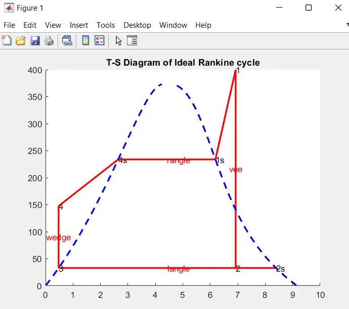
%ptotting T-S
figure(1)
hold on
plot([S1 S2],[T1 T2],'r','linewidth',2)
text(S1,T1,'1')
text(S1,T2,'2')
plot([S2 S2g],[T2 T2s],'r','linewidth',2)
text(S2g,T2s,'2s')
plot([S2g S3],[T2s T3],'r','linewidth',2)
text(S3,T3,'3')
plot([S3 S4],[T3 T4],'r','linewidth',2)
text(S4,T4,'4')
plot([S4 S1f],[T4 T1s],'r','linewidth',2)
text(S1f,T1s,'4s')
plot([S1f S1g],[T1s T1s],'r','linewidth',2)
text(S1g,T1s,'1s')
plot([S1g S1],[T1s T1],'r','linewidth',2)
plot(S_L,temp,'b','linestyle','--','linewidth',2)
plot(S_V,temp,'b','linestyle','--','linewidth',2)

%assigning the location

text(S1,(T1+T2)/2,'vee','HorizontalAlignment','center','color','r')
text((S2g+S2f)/2,T3,'langle','color','r')
text(S3,(T3+T4)/2,'wedge','HorizontalAlignment','center','color','r')
text((S1f+S1g)/2,T1s,'rangle','color','r')
title('T-S Diagram of Ideal Rankine cycle')
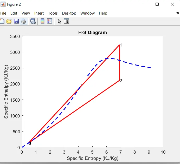
%plotting of H-S
figure(2)
hold on
plot([S1 S2],[H1 H2],'r','linewidth',2);
text(S1,H1,'1')
plot([S2 S3],[H2 H3],'r','linewidth',2);
text(S2,H2,'2')
plot([S3 S4],[H3 H4],'r','linewidth',2);
text(S3,H3,'3')
plot([S4 S1],[H4 H1],'r','linewidth',2);
text(S4,H4,'4')
plot(S_L, H_L,'b','linestyle','--','linewidth',2)
plot(S_V,H_V,'b','linestyle','--','linewidth',2)
title('H-S Diagram')
ylabel('Specific Enthalpy (KJ/Kg)')
xlabel('Specific Entropy (KJ/Kg)')

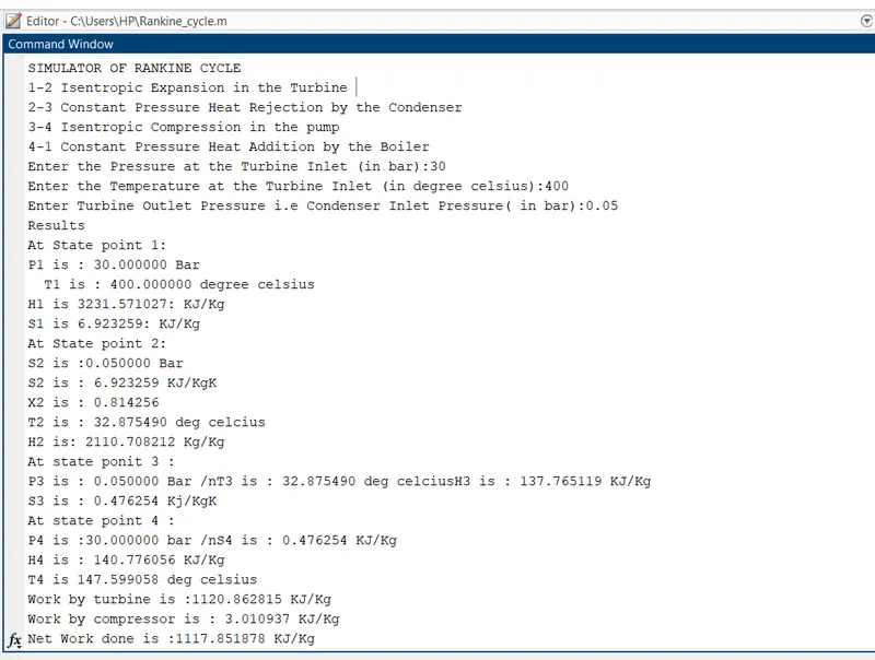
Output :

command window: