Week 4.1 - Genetic Algorithm
Generic algorithm was first introduced by Holland in 1975 and is a powerful stochastic search algorithm based on the mechanism of natural genetics and selection(Goldberg 1989)
Genetic algorithm starts with an initial set of random solution called Population.
Each inidividual in the population is called a chromosome representing a solution to the problem at hand.
The chromosome evolve through successive iteration called Generation.
During each generationthe chromosomes are evaluated using some measures of fitness.
To create the next generation, new chromosome called offspring are formed by either (i)merging two chromosomes from current generation using a crossover operator or (ii) modifying a chromosome using a mutation operator.
A new generation is formed by (i)selection according to the fitness values;some parents and offspring and(ii)rejecting others so as to keep the population size constant.
Fitter chromosomes have higher probabilities of getting selected.
After several generations, the algorithm converge to the best chromosome, which hopefuly represent the optimum or suboptimal solution to the problem.
A stalagmite is an upward-growing mound of mineral deposits that have precipitated from water dripping onto the floor of a cave. stalagmites have rounded or flattened tips.
Stalagmite function
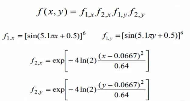
function [f]=stalagmite_func(Input_vector)
x=Input_vector(1);
y=Input_vector(2);
F1_X=(sin((5.1*pi*x)+0.5))^6;
F1_Y=(sin((5.1*pi*y)+0.5))^6;
F2_X=exp((-4*(log(2)).*(x-0.0667).^2)/0.64);
F2_Y=exp((-4*(log(2)).*(y-0.0667).^2)/0.64);
%Using the negative sign to find the global maxima point
f=-(F1_X*F1_Y*F2_X*F2_Y);
end
%Main code
%Creating the search space for thr function between 0 and 0.6
x=linspace(0,0.6,150)
y=linspace(0,0.6,150)
%Function is to iterate for 30 times
limits=30
%Converting the 1-D array into 2-D array using meshgrid
[xx yy]=meshgrid(x,y);
%Nested for loop for value input
for i=1:length(xx)
for j=1:length(yy)
Input_vector(1)=xx(i,j);
Input_vector(2)=yy(i,j);
f(i,j)= stalagmite_func(Input_vector);
end
end
%plotting the points
figure(1)
subplot(2,1,1)
% generating the surface
surf(xx, yy, -f);
%to remove the grid lines
shading interp
hold on;
xlabel('x value')
ylabel('y value')
plot3(xopt,yopt,-fval,'marker','o','MarkerSize',5,'MarkerFaceColor','r')
subplot(2,1,2)
plot(-fval);
xlabel('No_of_Iterations')
ylabel('Max_function_value')
%case-2 Bounding limits
%upper and lower limits specified in ga to reduce the search space within the boundary limit
%tic and tac commands are used to calculate the study time
tic
for k=1:limits
[input,fval(k)]=ga(@stalagmite_func,2,[],[],[],[],[0;0],[1;1]);
%calculating optimized value
xopt(k)=input(1);
yopt(k)=input(2);
end
study_time_2=toc;
%plotting the points
figure(2)
subplot(2,1,1)
%creating the surface
surfc(xx,yy,-f)
%To remove the grid lines
shading interp
hold on
plot3(xopt,yopt,-fval,'marker','o','MarkerSize',6,'MarkerFaceColor','r')
title('Bounded Input')
subplot(2,1,2)
plot(-fval)
xlabel('No of Iterations')
ylabel('Max function value')
%case-3 Increasing population
Increasing the population to increase the possibilities of finding the better fitness of the function.
options=optimoptions('ga')
options=optimoptions(options,'populationsize',150);
tic
for k=1:limits
[input,fval(k)]=ga(@stalagmite_func,2,[],[],[],[],[0;0],[1;1],[],[],options)
xopt(k)=input(1)
yopt(k)=input(2)
end
study_time_3=toc;
%plotting the points
figure(3)
%generating the surface
subplot(2,1,1)
surfc(xx,yy,-f)
%To remove the grid lines
shading interp
hold on
plot3(xopt,yopt,-fval,'marker','o','MarkerSize',6,'MarkerFaceColor','r')
title('Bounded_Input')
subplot(2,1,2)
plot(-fval)
xlabel('No of Iterations')
ylabel('Max function value')
problems faced while programing,
While plotting the surface, hold on command placing position is changed, so that 2d plot were generated.
While creating the surface, negative sign missed so the the plots generated in opposite side.
References:
1.https://www.youtube.com/watch?v=MLPHLm56inQ
2. https://www.youtube.com/watch?v=1i8muvzZkPw
3. https://www.youtube.com/watch?v=uQj5UNhCPuo
%stalagmite code

function [f]=stalagmite_func(Input_vector)
x=Input_vector(1);
y=Input_vector(2);
F1_X=(sin((5.1*pi*x)+0.5))^6;
F1_Y=(sin((5.1*pi*y)+0.5))^6;
F2_X=exp((-4*(log(2)).*(x-0.0667).^2)/0.64);
F2_Y=exp((-4*(log(2)).*(y-0.0667).^2)/0.64);
f=-(F1_X*F1_Y*F2_X*F2_Y);
end

%main code

clear all
close all
clc

%search space for the function
x=linspace(0,0.6,150);
y=linspace(0,0.6,150);
%function is to iterate for 50times.
limits=30;

%converting the one dimensional array into two dimension array
[xx yy]=meshgrid(x,y);

%Nested for loop for value input
for i=1:length(xx)
    for j=1:length(yy)
        Input_vector(1)=xx(i,j);
        Input_vector(2)=yy(i,j);
        f(i,j)= stalagmite_func(Input_vector);
    end
end

%Case-1 Satistical behaviour of Genetic Algorithm
tic
for k=1:limits
    [input, fval(k)]=ga(@stalagmite_func,2);
    xopt(k)=input(1);
    yopt(k)=input(2);
end

study_time_1=toc;

%plotting the points
figure(1)
subplot(2,1,1)
% generating the surface
surf(xx, yy, f);
%to remove the grid lines
shading interp
hold on;
xlabel('x value')
ylabel('y value')

plot3(xopt,yopt,-fval,'marker','o','MarkerSize',5,'MarkerFaceColor','r')
subplot(2,1,2)
plot(-fval);
xlabel('No_of_Iterations')
ylabel('Max_function_value')


%case-2 Bounding limits

tic
for k=1:limits
    [input,fval(k)]=ga(@stalagmite_func,2,[],[],[],[],[0;0],[1;1]);
    xopt(k)=input(1);
    yopt(k)=input(2);
end

study_time_2=toc;

figure(2)
subplot(2,1,1)
surfc(xx,yy,-f)
shading interp
hold on
plot3(xopt,yopt,-fval,'marker','o','MarkerSize',6,'MarkerFaceColor','r')
title('Bounded Input')
subplot(2,1,2)
plot(-fval)
xlabel('No of Iterations')
ylabel('Max function value')

%case-3 Increasing population

options=optimoptions('ga')
options=optimoptions(options,'populationsize',200);

tic
for k=1:limits
    [input,fval(k)]=ga(@stalagmite_func,2,[],[],[],[],[0;0],[1;1],[],[],options)
    xopt(k)=input(1);
    yopt(k)=input(2);
end

study_time_3=toc;

%plotting the points
figure(3)

%generating the surface
subplot(2,1,1)

surfc(xx,yy,-f)
hold on
%To remove the grid lines

shading interp

plot3(xopt,yopt,-fval,'marker','o','MarkerSize',6,'MarkerFaceColor','r')
title('Bounded_Input')
subplot(2,1,2)
plot(-fval)
xlabel('No of Iterations')
ylabel('Max function value')