Week 4.1 - Genetic Algorithm

Objective : Try to understand the concept of genetic algorithm by referring to varius sources before you attend this challenge. Look out for information regarding stalagmite function and ways to optimise it.

• Write a code in MATLAB to optimise the stalagmite function and find the global maxima of the function.
• Clearly expalin the concept of genetic algorithm in your own words and also explain the syntax for ga in MATLAB in your report.
• Make sure that your code gives the same output, even if it is made to run several times.
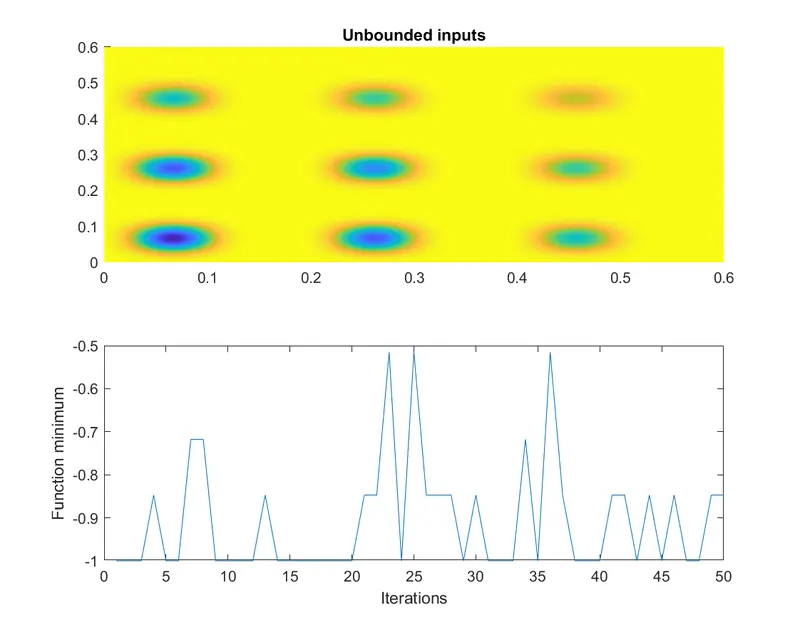
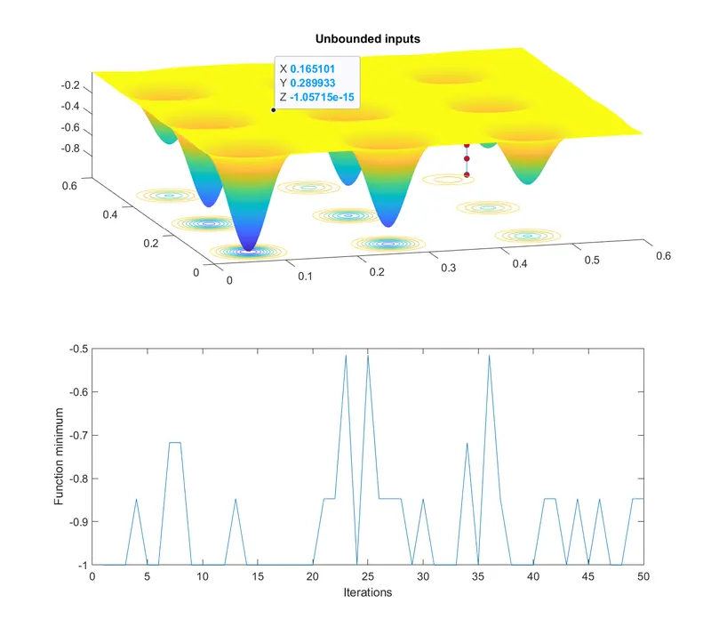
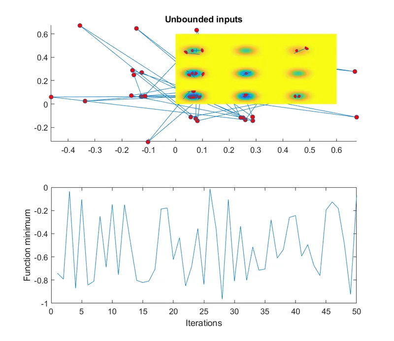
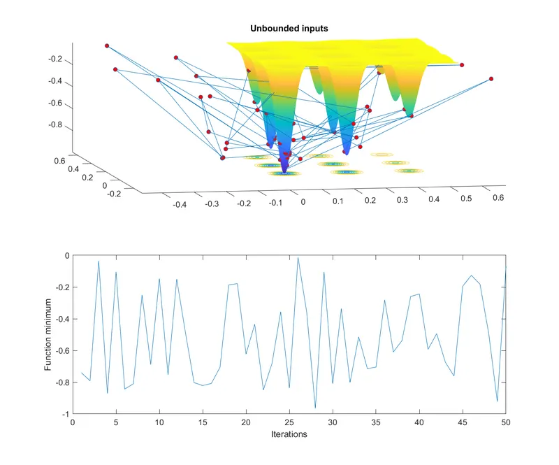
• Plot graphs for all 3 studies and for F maximum vs no. of iterations. Title and axes labels are a must, legends could be shown if necessary.

Theory: A genetic algorithm (GA) is a method for soving both constrained and unconstrained optimization problems based on natural selection process that mimics the biological evolution. The algorithm repeatedly modifies a population of indivisual solutions. At each step, the genetic algorithm randomly selects indivisuals from the current population and uses tham as parent to produce the children for the next generation. Over successive generations, the population "evolves" toward an optimal solution.In the followin area genetic algorithm is extensively used-

• Optimization
• Economics
• Neutral networks
• Image processing
• Machine learning
• DNA analysis
• Robot trajectory generation
• Parametric design of Aircraft.

Stalagmite function-

function [f]=stalagmite(V)
x = V(1);
y = V(2);

f1x=(sin((5.1*pi*x)+0.5))^6;
f1y=(sin((5.1*pi*y)+0.5))^6;
f2x=exp(-4*log(2)*(((x-0.0667)^2)/0.64));
f2y=exp(-4*log(2)*(((y-0.0667)^2)/0.64));

f=-(f1x*f1y*f2x*f2y);


MATLAB codes for GA-

clear all
close all
clc

x = linspace(0,0.6,150);
y = linspace(0,0.6,150);
num_cases = 50;
% Creating a 2D mesh
[xx, yy]=meshgrid(x,y);

% Evaluating the stalagmite function
 for i=1:length(xx)
  for j=1:length(yy)
    input_vector(1)=xx(i,j);
    input_vector(2)=yy(i,j);
    f(i,j)=stalagmite(input_vector);
  end
 end 

tic
% Study 1 - Statistical behavior
 for i = 1:num_cases
     [inputs, fopt(i)] = ga(@stalagmite, 2);
     xopt(i) = inputs(1);
     yopt(i) = inputs(2);
 end
Study1_time = toc;

 figure(1)
 subplot(2,1,1)
 hold on
 surfc(x,y,f)
 shading interp
 plot3(xopt,yopt,fopt,'marker','o','MarkerSize',5,'MarkerFaceColor','r')
 title('Unbounded inputs')
 subplot(2,1,2)
 plot(fopt)
 xlabel('Iterations')
 ylabel('Function minimum')

 tic
 % Study 2 - Statistical behavior with upper and lower bounds
  for i = 1: num_cases
      [Inputs, fopt(i)] = ga(@stalagmite,2,[],[],[],[],[0;0],[1;1]);
      xopt(i) = inputs(1);
      yopt(i) = inputs(2);
  end
Study2_time = toc;

figure(2)
subplot(2,1,1)
 hold on
 surfc(x,y,f)
 shading interp
 plot3(xopt,yopt,fopt,'marker','o','MarkerSize',5,'MarkerFaceColor','r')
 title('Unbounded inputs')
 subplot(2,1,2)
 plot(fopt)
 xlabel('Iterations')
 ylabel('Function minimum')

Outputs: