Week 3 - Solving second order ODEs

Objective: Write a program that solves the 2nd order ODE.

Theory: A 2nd order ordinary differential eqution is an equation in which any derivatives with respect to the independent variable have order no greater than 2. Ordinary differential equtions helps us to solve the many enginerring problems such as harmonic motions,vibrations,damping and also used to model many engineering systems.

The following ODE represents the equation of motion of a simple pendulum with damping-

In the above equation,

g = gravity in m/s2,

L = length of the pendulum in m,

m = mass of the ball in kg,

b=damping coefficient.

Inputs:

L=1 metre,

m=1 kg,

b=0.05.

g=9.81 m/s2.

Initial condition:

Angular displacement=0,

Angular velocity=3 rad/sec at time t=0

The motion is simulated between 0-20 sec.

MATLAB codes for solving ODE:

clear all
close all
clc

% Damping coefficient
b=0.05;
% Acceleration due to gravity in m/s2
g=9.8;
% Length of the pendulum in m
l=1;
% Mass in kg
m=1;

% Initial condition
theta=[0;3];

% Time points
t_span=linspace(0,20,300);

% Solve ODE
[t,results]=ode45(@(t,theta) ode_func(t,theta, b,g,l,m),t_span,theta);


%Animating the motion of pendulum

figure(2)
ct=1;

for i = 1:length(t_span)
    
        x0 = 0;
        y0 = 0;

        x1 = l*sin(results(i,1));
        y1 = -l*cos(results(i,1));

      

        % Plotting

        plot([0 0],[-1.5 0.5])
        hold on
        plot([x0 x1],[y0 y1],'linewidth',3,'Color','b')
        axis([-1.5 1.5 -1.5 0.5])
        plot(x1, y1,'o','Markersize',20,'Color','r')
        pause(0.0001)
        M(ct)=getframe(gcf);
        hold off
        ct=ct+1;

end

figure(1)
plot(t,results(:,1))
hold on
plot(t,results(:,2))
ylabel('Velocity(Red) & Displacement(Blue)')
xlabel('time')

%making the video file

movie(M)
videofile = VideoWriter('ode_1.avi');
open(videofile)
writeVideo(videofile,M)
close(videofile)


ODE function are given below-

 function[dtheta_dt]= ode_func(t,theta,b,g,l,m)
 
   theta1 = theta(1)
   theta2 = theta(2)
   dtheta1_dt = theta2;
   dtheta2_dt = -(b/m)*theta2 -(g/l)*sin(theta1);
   dtheta_dt = [dtheta1_dt; dtheta2_dt];
end

 

Output:

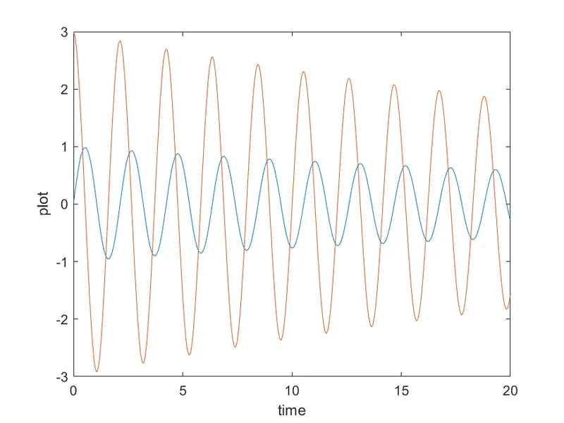
Video link:

https://youtu.be/TUnM1sONkEc

Explationation:

1) In above program fixed parameters are length,mass,damping coefficient and g.

2) Time and angles are given as initial condition.

3) In the tspan command, 200 values are taken in between 0 to 20 times period.

4) Using ode 45 command ODE function is introduced.

5) Using the plot command velocity and displacement is plotted in y-axis against time in the x-axis.

6) Using for loop command yhe mass at various points and various times are marked in the graph.

7) Using movie command the plot is saved as avi. file.