Week 4.1 - Genetic Algorithm
The codes :
1) Function code for stalagmite function :
function [sf] = stalagmite(input_vector)

% inputs
x = input_vector(1);
y = input_vector(2);

% given formula for the stalagmite function
% f(x,y) = [sin(5.1*pi*x+0.5)]^6 * [sin(5.1*pi*y+0.5)]^6 *
% exp[-4*log(2)*((x-0.0667)^2/0.64))] * exp[-4*log(2)*((y-0.0667)^2/0.64))]
term1 = (sin(5.1*pi*x+0.5))^6;
term2 = (sin(5.1*pi*y+0.5))^6;
term3 = exp(-4*log(2)*((x-0.0667)^2/0.64));
term4 = exp(-4*log(2)*((y-0.0667)^2/0.64));

sf = -(term1*term2*term3*term4);

end
2) Optimization code with genetic algorithm for stalagmite function :
close all
clear all
clc

% defining our search space
x = linspace(0,0.6,150);
y = linspace(0,0.6,150);

% creating a 2d mesh
[xx , yy] = meshgrid(x ,y);

% evaluating the stalagmite function
for i = 1:length(xx)
    for j = 1:length(yy)
        input_vector(1) = xx(i,j);
        input_vector(2) = yy(i,j);
        f(i,j) = stalagmite(input_vector);
    end
end

% plotting
surfc(xx,yy,-f)
xlabel('x value')
ylabel('y value')
shading interp

% performing ga
[inputs,fval] = ga(@stalagmite,2);
3) Code for studies of the optimization :
close all
clear all
clc

% defining our search space
x = linspace(0,0.6,150);
y = linspace(0,0.6,150);
num_case = 50

% creating a 2d mesh
[xx , yy] = meshgrid(x ,y);

% evaluating the stalagmite function
for i = 1:length(xx)
    for j = 1:length(yy)
        input_vector(1) = xx(i,j);
        input_vector(2) = yy(i,j);
        f(i,j) = stalagmite(input_vector);
    end
end

%Study 1:Statistical behaviour
tic
for i = 1:num_case
    [inputs , fopt(i)] = ga(@stalagmite,2);
    xopt(i) = inputs(1);
    yopt(i) = inputs(2);
end
study1_time = toc
% ploting
figure(1)
subplot(2,1,1)
hold on
surfc(x,y,-f)
plot3(xopt,yopt,-fopt,'marker','o','markersize',5,'markerfacecolor','r')
xlabel('x value')
ylabel('y value')
shading interp
title('Unbound inputs')
subplot(2,1,2)
plot(-fopt)
xlabel('Iterations')
ylabel('Function minimum')

%Study 2:for the optimization
tic
for i = 1:num_case
    [inputs , fopt(i)] = ga(@stalagmite,2,[],[],[],[],[0;0],[0.4;0.4]);
    xopt(i) = inputs(1);
    yopt(i) = inputs(2);
end
study2_time = toc
% ploting
figure(2)
subplot(2,1,1)
hold on
surfc(x,y,-f)
plot3(xopt,yopt,-fopt,'marker','o','markersize',5,'markerfacecolor','r')
xlabel('x value')
ylabel('y value')
shading interp
title('Bound inputs')
subplot(2,1,2)
plot(-fopt)
xlabel('Iterations')
ylabel('Function maximum')

%study 3:increasing ga iteratiom
options = optimoptions('ga')
options = optimoptions(options,'populationsize',500);
tic
for i = 1:num_case
    [inputs , fopt(i)] = ga(@stalagmite,2,[],[],[],[],[0;0],[0.4;0.4],[],[],options);
    xopt(i) = inputs(1);
    yopt(i) = inputs(2);
end
study3_time = toc
% ploting
figure(3)
subplot(2,1,1)
hold on
surfc(x,y,-f)
plot3(xopt,yopt,-fopt,'marker','o','markersize',5,'markerfacecolor','r')
xlabel('x value')
ylabel('y value')
shading interp
title('Bound inputs with increased population')
subplot(2,1,2)
plot(-fopt)
xlabel('Iterations')
ylabel('Function maximum')
Out put & plots :
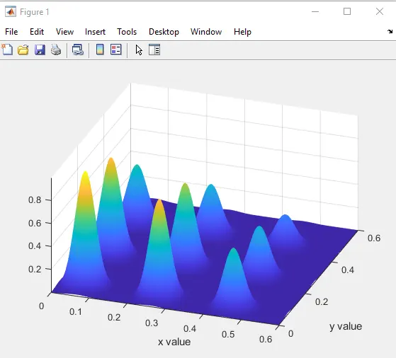
1) Optimization of stalagmite function (op of code no 2):
2 ) Optimization studies of stalagmite function with F maximum vs no. of iterations (op of code no 3):
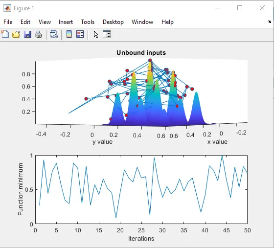
study 1:
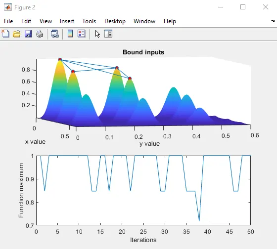
study 2:
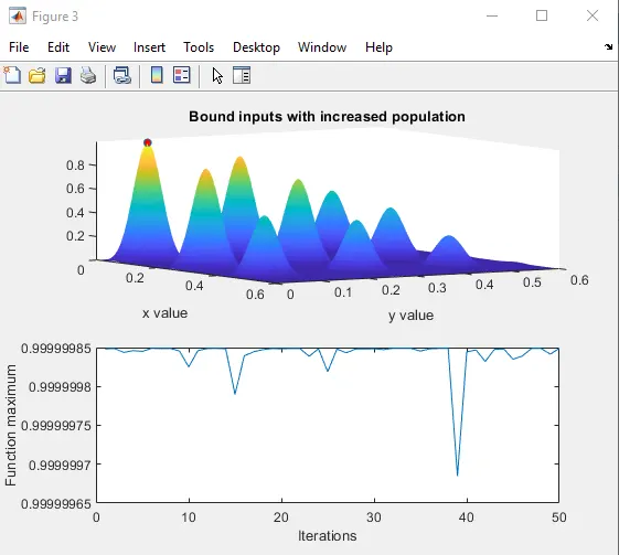
study 3:
Report :
what is genetic algorithm ?
A: A genetic algorithm(ga) is a metaheuristic inspired by the process of natural selection that belongs to the larger class of Evolutionary algorithms (EA). Genetic algorithms are commonly used to generate high-quality solutions to optimization and search problems by relying on biologically inspired operators such as mutation , crossover and selection. Some examples of GA applications include optimizing decsion trees for better performance, automatically solve sudoku puzzles , hyperparameter optimization etc.
what is optimization ?
A: The purpose of optimization is to achieve the best design relative to a set of prioritized criteria or constraints.These include maximizing factors such as productivity, strength, reliability, longevity, efficiency, and utilization. This decision-making process is known as optimization.
The concept of genetic algorithm(how it works) :
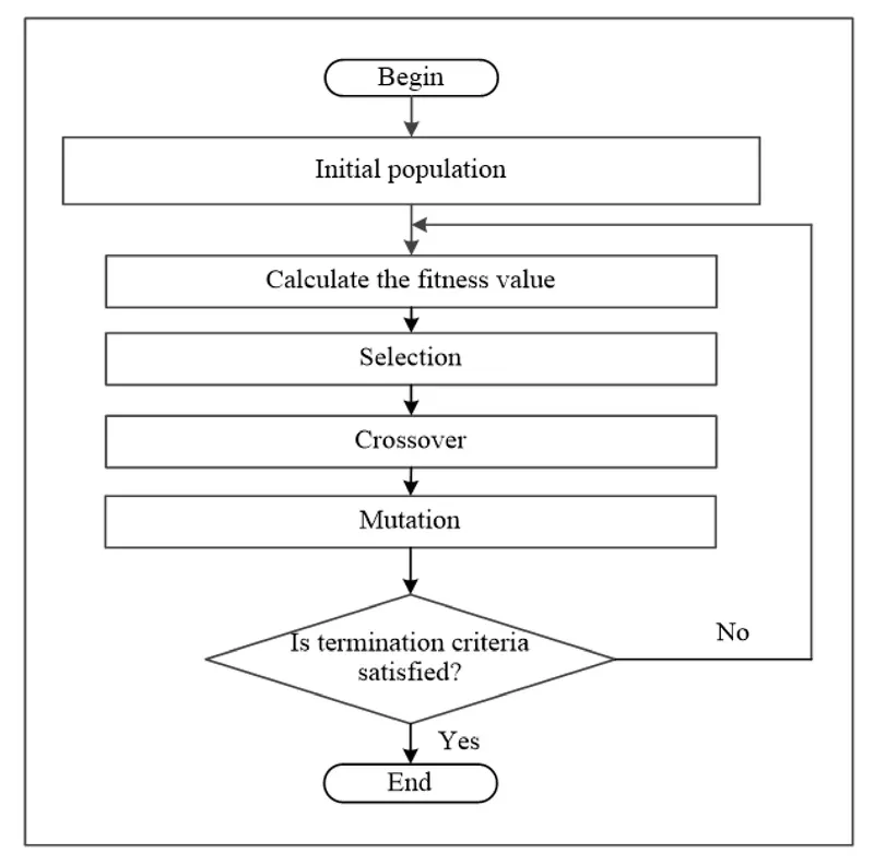
Genetic Algorithm (GA), first introduced by Holland (1975), is a powerful stochastic search algorithm based on the mechanisms of natural genetics and selection (Goldberg 1989). A general description of GA is as follows:
# Genetic algorithm starts with an initial set of random solutions called population.
# Each individual in the population is called a chromosome representing a solution to the problem at hand.
# The chromosomes evolve through successive iterations, called generations.
# During each generation, the chromosomes are evaluated using some measures of fitness.
# To create the next generation, new chromosome, called offspring, are formed by either (a) merging two chromosomes from current generation using a crossover operator or (b) modifying a chromosome using a mutation operator.
# A new generation is formed by (a) selecting,according to the fitness values, some of the parents and offspring and (b) rejecting others so as to keep the population size constant.
# Fitter chromosomes have higher probabilities of being selected.
# After several generations, the algorithms converge to the best chromosome, which hopefully represents the optimum or suboptimal solution to the problem
syntax for genetic algorithm :
x = ga(fun,nvars)
x = ga(fun,nvars,A,b)
x = ga(fun,nvars,A,b,Aeq,beq)
x = ga(fun,nvars,A,b,Aeq,beq,lb,
x = ga(fun,nvars,A,b,Aeq,beq,lb,
x = ga(fun,nvars,A,b,Aeq,beq,lb,
x = ga(fun,nvars,A,b,[],[],lb,ub,
x = ga(fun,nvars,A,b,[],[],lb,ub,
x = ga(problem)
[x,fval] = ga(___)
[x,fval,exitflag,output] = ga(___)
[x,fval,exitflag,output,
syntax explanation :
# x = ga(fun,nvars,A,b) finds a local minimum x to fun, subject to the linear inequalities A*x<=b ga evaluates the matrix product A*x as if |x| is transposed (A*x')
# x = ga(fun,nvars,A,b,Aeq,beq) finds a local minimum x to fun ,subject to the linear equalities Aeq*x=beq and A*x<=b(Set A=[] and b=[] if no linear inequalities exist.) ga evaluates the matrix product Aeq*x as if x is transposed (Aeq*x')
# x = ga(fun,nvars,A,b,Aeq,beq,lb,
# x = ga(fun,nvars,A,b,Aeq,beq,lb,
# x = ga(fun,nvars,A,b,Aeq,beq,lb,
# x = ga(fun,nvars,A,b,Aeq,beq,lb,
# x = ga(problem)finds the minimum for problem,a structure described in problem.[x,fval] = ga(___)for any previous input arguments, also returns fval, the value of the fitness function at x.
# [x,fval,exitflag,output ] = ga(___)also returns exitflag an integer identifying the reason the algorithm terminated,output a structure that contains output from each generation and other information about the performance of the algorithm.
# [x,fval,exitflag,output,
code explanation :
1) Function code for stalagmite function :
- I have created a function code , that can take inputs of two vectors and will provide a solution for creating a stalagmite structure .
- Input vectors x , y are provided to the code.
- Finally used a provided formula to create the solution for creating a stalagmite structure.
2) Optimization code with genetic algorithm for stalagmite function :
- started the program with clear all , close all , clc.
- with the linspace command i have created two vectors.
- with the command 'meshgrid' i have created a 2d mesh from the two vectors x,y .
- with the use of for loop , i have created two desired vectors . and by calling the stalagmite function
- then by calling the stalagmite function and providing the function with previously created vectors , i have achived the solution for creating the stalagmite structure .
- after that with the help of 'surfc' command , i have ploted the stalagmite structure.
- then performed genetic algorithm with the stalagmite function by using inbuilt command 'ga'.
3) Code for studies of the optimization :
study 1 :
- in this part , we are studying the statistical behaviour of the ga,we are performing ga 50 times , and studying the outputs.
- performing ga with the stalagmite function for 50 times.
- storing the values of x,y for all the ga performed and stored the data in two variables x_opt ,y_opt
- with the 'tic' & 'toc' command we got to know the time it took for the operation.
- then by plotting the stalagmite structure , output for every ga run , and optimum function value that ga predicts for every ga run we can learn that how the ga is performing.
study 2 :
- we are performing the same code as the study 1 , but only with one modification ,this time we are providing upper and lower limit for the minimum value of x,y.
study 3 :
- in this code with the addition of providing upper and lower limit for the minimum value of x,y , we are also altering with the size of population for the ga.
Findings from the above studies :
- from study 1 , we found the minimum value for x,y , but the value was unusable because of the absence of upper and lowe limit for x,y , the ga was providing values outside the stalagmite function.
- in the study 2 , we provide upper and lower limit to the ga ,and we got the values for x,y inside the stalagmite function , but still we needed to improve , because there was too much minimum values for x,y.
- in the study 3 , we altered the search space for the ga , [depending upan the problem , we have to provide an educational guess for the search space] , here we increased the number of samples/population for the ga , beacuse we cant find global minima with less number of population.
- we got to know that with increased population , the ga takes more time to give the output.
References :
- https://in.mathworks.com/discovery/genetic-algorithm.html
- https://www.youtube.com/watch?v=MLPHLm56inQ
- https://www.youtube.com/watch?v=1i8muvzZkPw
- https://www.researchgate.net/post/How_to_write_genetic_algorithms_codes_in_Matlab