Week 3 - Solving second order ODEs

The code :

1) Function code for solving ODE :

% function code

function [dtheta_dt] = ode_func(t,theta,b,g,l,m)

theta1 = theta(1);
theta2 = theta(2);
dtheta1_dt = theta2;
dtheta2_dt = -(b/m)*theta2 - (g/l)*sin(theta1);
dtheta_dt = [dtheta1_dt ; dtheta2_dt];
end

2) ODE solving and pendulum simulation code :

close all
clear all
clc

% Given values for the pendulum
b = 0.05; % damping coefficient
g = 9.81; % gravity in m/s2
l = 1; %  length of the pendulum in m
m = 1; % mass of the ball in kg

% initial condition of the pendulum
% initially angular displacement is'0' & angular velocity is '3'  
ini_c = [0;3];

% time span(in seconds) 
t_span = linspace(0,20,700);

% solving the ode
[t,results] = ode45(@(t,theta) ode_func(t,theta,b,g,l,m),t_span,ini_c);
pos_pe_wrtt = results(:,1);

% plotting the result of the ode
figure(1)
plot(t,results(:,1))
hold on
plot(t,results(:,2))
xlabel('plot')
ylabel('time')
legend('angular displacement ','angular velocity')

% animating the motion of the pendulum
ct = 1;
for a = 1:length(pos_pe_wrtt);
    Pos_pe_wrtt = pos_pe_wrtt(a);

% defining the coordinates 
x0 = 0;
y0 = 0;
x1 = l*sin(Pos_pe_wrtt);
y1 = -l*cos(Pos_pe_wrtt);

% plotting the coordinates & the pendulum
figure(2)
plot([-1,1],[0,0],'LineWidth',5)
hold on
plot([x0,x1],[y0,y1],'LineWidth',3)
hold on
plot(x1,y1,'o','MarkerSize',25,'MarkerFaceColor','g')
axis([-1.5 1.5 -1.5 1.5])
pause(0.03)
hold off
M(ct) = getframe(gcf);
ct = ct+1;
end

% creating the movie
movie(M)
videofile = VideoWriter('solving_second_order_ODE_pendulum_animation.avi','Uncompressed AVI');
open(videofile)
writeVideo(videofile,M)
close(videofile)

Out put :

1) ODE output representation in a plot :

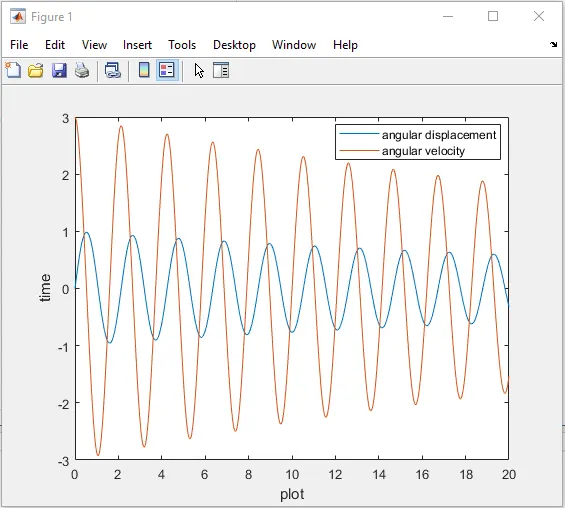
2) Pendulum animation :

youtube link - https://youtu.be/PRYqNwHZHAY

Report :

Differential equation :

A differential equation is an equation that relates one or more functions and their derivatives . In applications, the functions generally represent physical quantities, the derivatives represent their rates of change, and the differential equation defines a relationship between the two.

Second order ordinary differential equation :

A second order ordinary differential equation is an ordinary differential equation in which any derivatives with respect to the independent variable have order no greater than 2">2.

Pendulum :

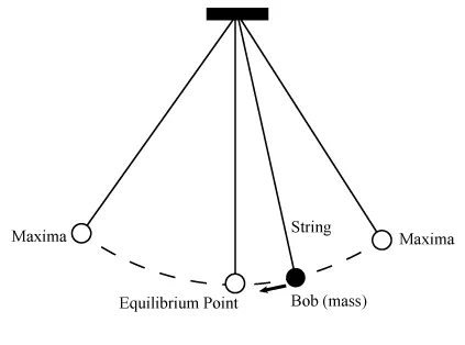
-A pendulum is a weight hung from a stationary point in a way that allows it to swing freely back and forth. A simple pendulum is one where the pendulum bob is treated as a point mass, and the string from which it hangs is of negligible mass. Simple pendulums are interesting from a physics perspective because they are an example of simple harmonic motion.

-Simple harmonic motion is any periodic motion where a restoring force is applied that is proportional to the displacement and in the opposite direction of that displacement.

-When you lift a pendulum to one side, the force of gravity wants to pull it back down, and the tension in the string wants to pull it left (or right). These combined forces work together to pull it back towards the middle (the equilibrium position). Ultimately, upon reaching the middle, the pendulum's velocity has increased, so it continues past the equilibrium position and off to the other side. This pattern then continues.

-The way a pendulum moves depends on the Newtons second law. When this law is written down, we get a second order Ordinary Differential Equation that describes the position of the "ball" w.r.t time.

Provided ode :

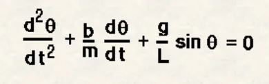
- This is a second order ode.

- In order to solve a second order ode , first we need to break it down to set of first order ode.

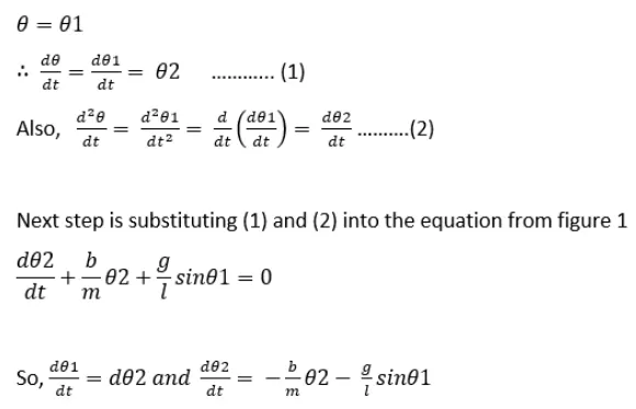
-From the above two first order ode , we need to create a solution vector .

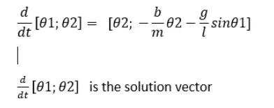
-With the use of matlab inbuilt solver , we can solve the second order ode from this above solution vector.

Explanation of the code :

strategy for the code :

- First we need to solved the second order ode with the help of inbuilt matlab solvers .

- After solving the ode with the provided time span , we will get angular displacement and angular velocity w.r.t time.

-We will create a plot for each angular displacement , and to make an animation out of the plots , we will stich all the plots.

1)Function code explanation :

- I have created a function code , that can take inputs of provided gravity , mass of the ball , length of the string and damping co-efficient.

- Then i have written the 'solution vector' of the second order ode , and ended the function

- i will use this function inside the main program to solve the second order ode.

2) ODE solving and pendulum simulation code explanation :

- pendulum specification , time span and initial angular displacement and velocity is provided.

- with the linspace command , i have divided the 20 second time span to 700 parts.

- then with the help of 'ode 45' solver , i have solved the second order ode , by calling the function code that i created earlier.

- As a result , i got angular displacement and angular velocity w.r.t the time 20 seconds , as i have divided the 20 seconds in to 700 parts , i got 700 values for angular displacement & velocity , each represent a different position of the pendulum at a different time.

- then with the plot command i ploted the angular displacement & velocity plot w.r.t time.

Animating the motion of the pendulum :

- as i have 700 values for angular displacement , i need a plot for each angular displacement for the animation , and for that purpose i have used a for loop , because i need to perform the task again and again for a known interval.

- 'pos_pe_wrtt' have 700 values of angular displacement . and 'a' represents the interval , that how many times the for loop will execute.

- then i have defined the co-ordinated for the pendulum , as one point of the pendulum is fixed the co-ordinate will be (0,0) and for the end point , the co-ordinates are derived using basic trogonometry formula.

- with the plot command , i ploted the surface , in which the pendulum is suspended and again with the plot command i joined the co-ordinated of the pendulum .at the end point of the pendulum , i have created a ball/mass using plot command .

- then i have provided the axis and a pause interval , the loop will execute with the provided pause interval.

Making the movie :

- The animation is successfully created , but i need a video file out of it.

- for that i have saved individual frames in a array 'm(ct)' , here 'ct' stands for individual frames.and used the syntax 'getframe(gcf)'. because each plot is a figure , the 'getframe' command collect all the figureas.

- 'ct = ct + 1' because the counter needs to increment each time the loop is executed.

- after this i have ended the for loops.

- at the end i have used the syntax 'movie(M)' , this will generate a movie with the array 'M'( which contains all the frames )

- to save the frames in a file , i have created a video file with the command 'videowriter' . and provided the file name and profile.

-and then i have opened the videofile that i just created and with the command 'writevideo' i write all the frames/ 'M' array in the video file.

and then closed the video file.

Error faced while programming :

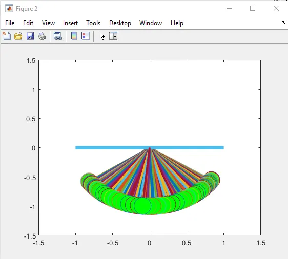
- this was happening because of the abscence of 'hold off' command .