Week 4.1 - Genetic Algorithm
AIM: TO STUDY OPTIMISATION BY USING GEOMETRIC ALGORITHM IN MATLAB
FORMULA:
f(x,y)=f1,xf2,xf1,yf2,y
01:f1.x=[sin(5.1pix+0.5)]^6
02:f1.y=[sin(5.1piy+0.5)]^6
03:f2.x=exp[-4ln(2)(x-0.0667)^2/0.64]
04:f2.y=exp[-4ln(2)(y-0.0667)^2/0.64]3:
OBJECTIVE:
1:TO THE CODE FOR OPTIMIZATION OF THE STALAGMITE AND FIND GLOBAL MAXIMA.
2:EXPLANATION OF THE GEOMATRIC ALGORITHM AND SYNTAX USED FOR IT.
3:CODE MUST GIVE THE SAME OUTPUT EVEN IF IT IS MADE TO RUN SEVERAL TIME.
4:GRAPH OF ALL THREE STUDIES MUST HAVE LABELS AND TITLES.
5:MENTION THE ERROR COMMITED DURING PROGRAMMING AND STEP TAKEN TO CORRECT IT.
INTRODUCTION:
WHAT IS OPTIMIZATION?
Mathematical optimization (alternatively spelled optimisation) or mathsatical programning is the selection of
a best elenent (with regard to some criterion) from some set of available alternatives. Optiization probless
of sorts arise in all quantitative disciplines fron computer science and engineering to operations research and
economics, and the development of solution methods has been of interest in mathematics for centuries.
In the field of engineering and research we need to find the maximun and minimun values of specific parameters
to evaluate the systens for better performance. In such situations it becomes very important to find the
minimun and maxinun values of the given parameters within the specific range of operation.
This whole process of calculating the required minimum or maximum values (optimum values of parameter for
optinun results of the systen.) of the specific paraseter for the evaluation of the system is called as
optimization.
Optimization includes finding best available values of some objective function given a defined domain (or
input), including a variety of different types of objective functions and different types of domains.
a best elenent (with regard to some criterion) from some set of available alternatives. Optiization probless
of sorts arise in all quantitative disciplines fron computer science and engineering to operations research and
economics, and the development of solution methods has been of interest in mathematics for centuries.
In the field of engineering and research we need to find the maximun and minimun values of specific parameters
to evaluate the systens for better performance. In such situations it becomes very important to find the
minimun and maxinun values of the given parameters within the specific range of operation.
This whole process of calculating the required minimum or maximum values (optimum values of parameter for
optinun results of the systen.) of the specific paraseter for the evaluation of the system is called as
optimization.
Optimization includes finding best available values of some objective function given a defined domain (or
input), including a variety of different types of objective functions and different types of domains.
WHAT IS GENETIC ALGORITHM IN MATLAB?
A genetic algorithm is a search heuristic that is inspired by Charles Darwin's theory of natural evolution.
This algorithm reflects the process of natural selection where the fittest individuals are selected for
reproduction in order to produce offspring of the next generation.
This algorithm reflects the process of natural selection where the fittest individuals are selected for
reproduction in order to produce offspring of the next generation.
Same is done in the field of technical research and development. To dvelope or evaluate the performance of the
systen we need to select the optimum values of the specific parameters. For determining the optimum values,
Is done in the matlab using Geometric Algorithm (ga).
These algorithm are designed to solve Geometric Problems. They requires in-depth knowledge of different
mathematical subjects like combinatorics, topology, algebra, differential geometry etc.
A genetic algoritha (GA) is a method for solving both constrained and unconstrained optimization problems based
on a natural selection process that mimics biological evolution. The algorithm repeatedly modifies a population
of individual solutions. At each step, the genetic algorithm randomly elects individuals from the current
population and uses the as parents to produce the children for the next generation. Over successive
generations, the population evolves toward an optimal solution.
You can apply the genetic algorithn to solve problems that are not well suited for standard optimization algorithm including problems in which the objective function is discontinuous, non-differentiable,stochastic, or highly non linear.
FOR EXAMPLE:Comparing the slope of two line, finding equation of the plane etc.
Now let us understand genetic algoritm in detail
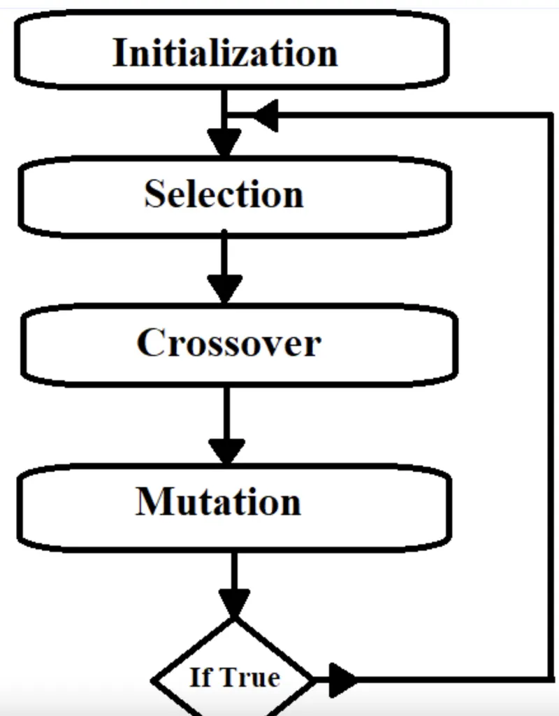
DIAGRAM SHOWS THE STEP TAKEN IN GENETIC ALGORITHM
INITIALIZATION:
In this stage we need to start the process by dividing or sorting the population we have into the diggeren
categories so that we can use the best of the data available for the optinization
categories so that we can use the best of the data available for the optinization
SELECTION:
In this stage we have to select the different variables of the data under consideration so that we can use
for the process of the optimization. Selection is based onthe fitness function. We call this selected set
data or variables as chromozones. We perform some operations on the selected chromozones.
CROSSOVER:
In this stage we have to select the different variables of the data under consideration so that we can use
for the process of the optimization. Selection is based onthe fitness function. We call this selected set
data or variables as chromozones. We perform some operations on the selected chromozones.
CROSSOVER:
While performing this actions after seletion of chromozones we exchange the characteristics of both the
chromozones with one another to obtain the best of the new set of chromozones which is always a better
alternative when compared to the best of the old set of chronozones,this process is called as crossover.
chromozones with one another to obtain the best of the new set of chromozones which is always a better
alternative when compared to the best of the old set of chronozones,this process is called as crossover.
MUTATION:
Addition of the new characteristics to the new set of chromoxones in order to level up the fitness of the
chromozoens so they can survive and sustain against the worst of the situations, this process is called as mutation.
Same cycle is repeated unless and until true condition of the 'stop' is attempted.
chromozoens so they can survive and sustain against the worst of the situations, this process is called as mutation.
Same cycle is repeated unless and until true condition of the 'stop' is attempted.
The genetic algorithm differs from a classical, derivative-based, optimization algorithm in two main ways, as summarized in the following table.
| Classical Algorithm | Genetic Algorithm |
|---|---|
|
Generates a single point at each iteration. The sequence of points approaches an optimal solution. |
Generates a population of points at each iteration. The best point in the population approaches an optimal solution. |
|
Selects the next point in the sequence by a deterministic computation. |
Selects the next population by computation which uses random number generators. |
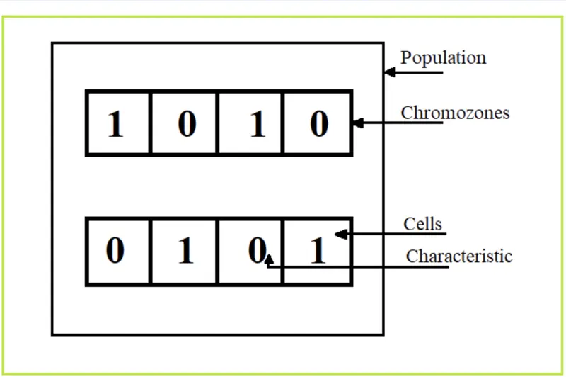
DIAGRAM SHOWS THE BASIC OF THE GENETIC ALGORITHM
SYNTEX FOR GA:
Now let us take an example to study and understand the syntex of genetic algorithm in matlab :
in our program we are implimenting the syntex of GA for minimizing the nonlinear function with integer constraints.
EXAMPLE:
We have following data available for the minimization.
01. min fun(x) i.e. F = (f1*f2*f3*f4)
Assume for f1, f2, 13 and f4 equations e1, e2, e3 and e4 are given respectively defined by the variables such
as'x' and 'y'
[We have function f(x) and we have to determine the minima of it. For mixima we have to multiply the
function by-ve. Therefore we programmed the function program for the objective function named as stalagmite]
01. min fun(x) i.e. F = (f1*f2*f3*f4)
Assume for f1, f2, 13 and f4 equations e1, e2, e3 and e4 are given respectively defined by the variables such
as'x' and 'y'
[We have function f(x) and we have to determine the minima of it. For mixima we have to multiply the
function by-ve. Therefore we programmed the function program for the objective function named as stalagmite]
02. s.t. Ax <= b i.e. Linear or Non-linear inequality constraints.
A = [];
b = [];
A = [];
b = [];
[while solving the example we need to convert the inequality constraint into the equality constraint]
03. Aeqx = beq i. e. Linear or Non-linear equality constraints.
Aeq = [];
beq = [];
[while solving remember that equality constraints are always subjected to (s.t.) inequality constraints.]
Aeq = [];
beq = [];
[while solving remember that equality constraints are always subjected to (s.t.) inequality constraints.]
04. LB <= X <= UB i. e. there are lower and upper bounds on the x
[Lower bounds = (0:0) and Upper bounds = (0.1:0.1) .]
[Lower bounds = (0:0) and Upper bounds = (0.1:0.1) .]
05. As given in the data we have two variables x and y.
Therefore number of variables are 2.
06. ga is the inbuilt command in the matlab for solver.
Syntax:
x = ga(fun,2,A,b,Aeq, beq, lb, ub, nonlcon, Intcon)
x = ga(fun,2,A,b,Aeq, beq, lb, ub, nonlcon, Intcon)
Application of syntax:
[inputs, fopt(i)] = ga(@stalagmite,2,[],[],[],[],[0:0], [0.1:0.1]) ;
[inputs, fopt(i)] = ga(@stalagmite,2,[],[],[],[],[0:0], [0.1:0.1]) ;
2. Problem Statement:
To understand the concept of genetic algorithm, optimize the stalagmite function and find
the global maxima of the function. By using Geometric algorithm optimize the stalagmite function.
the global maxima of the function. By using Geometric algorithm optimize the stalagmite function.
PROGRAM1 FOR MAXIMA OF THE FUNCTION STALAGMITE.M
clear all
close all
clc
% Defining our search space
x=linspace(0,0.6,150)
y=linspace(0,0.6,150)
%creating the two dimenasional mesh
[xx,yy]=meshgrid(x,y);
%evaluating the stalagmite function
for i=1:length(xx)
for j=1:length(yy);
input_vector(1)=xx(i,j);
input_vector(2)=yy(i,j);
f(i,j)=stalagmite(input_vector);
end
end
surfc(xx,yy,f)
shading interp;
[inputs,fval]=ga(@stalagmite,2);
figure(1)
surfc(x,y,f)
shading interp
Detailed Explanation of the program:
-starting the program with the usual coomand clear all,close all,clc .
-defining the search space
-x=linspace(0,0.6,150)
defining the element of the data of the space in which we have to carry out our optimization so we are firstly defining the x coordinate in the 2d space.
-y=linspace(0,0.6,150)
secondly we are defining the y cordinate of 2D space
- Creating a 2D mesh
Since we defined the x and y coordinates of the data as the row vectors, it is necessary to convert these
vectors into 2D mesh which will give us the 2D space for the operation. This is done by using the
meshgrid command in matlab.
Since we defined the x and y coordinates of the data as the row vectors, it is necessary to convert these
vectors into 2D mesh which will give us the 2D space for the operation. This is done by using the
meshgrid command in matlab.
- [xx yy] = meshgrid(x,y);
- Evaluating the stalagmite function
Stalagmite is the mathematical model which helps us to determine the 2D and 3D meshing of the data for the
given set of equations.
Stalagmite is the mathematical model which helps us to determine the 2D and 3D meshing of the data for the
given set of equations.
-for 1 = 1: length (xx);
Starting of for loop' selecting the values of x-axis of the 2D mesh.
Starting of for loop' selecting the values of x-axis of the 2D mesh.
- for j = 1: length(yy);
Starting of second "for loop' selecting the values of y-axis of the 2D mesh.
Starting of second "for loop' selecting the values of y-axis of the 2D mesh.
- input_vec(1) = xx(i,j);
Saving the values of the X-axis of the 2D mesh under the variable input_vec(1), which is used to give
input values of the variable x of the governing equations of the optimization.
Saving the values of the X-axis of the 2D mesh under the variable input_vec(1), which is used to give
input values of the variable x of the governing equations of the optimization.
- input_vec(2) = yy(i,j);
Saving the values of the y-axis of the 2D mesh under the variable input_vec(2), which is used to give
input values of the variable y of the governing equations of the optimization.
Saving the values of the y-axis of the 2D mesh under the variable input_vec(2), which is used to give
input values of the variable y of the governing equations of the optimization.
-f(i,j)=stalagmite(input_vector)
Entering the stalagmite function for the governing equations of the optimization, under the variable
defined by the coordinates (i,j) values.
- end
End of first 'for loop'
defined by the coordinates (i,j) values.
- end
End of first 'for loop'
- end
End of second 'for loop'
- % surfc (xx, yy, f)
- % shading interp
- (inputs, fval] = ga(@F_stalagmite, 2) ;
End of second 'for loop'
- % surfc (xx, yy, f)
- % shading interp
- (inputs, fval] = ga(@F_stalagmite, 2) ;
"ga' is the inbuilt command in the matlab that defines the geometric algorithm and by using it we can find
out the maxima values for the given data, helping the optimization of the given problem. The '2' denotes the
total number of variables used in the stalagmite function for the optimization.
out the maxima values for the given data, helping the optimization of the given problem. The '2' denotes the
total number of variables used in the stalagmite function for the optimization.
-figure(1)
surfc(x,y,f)
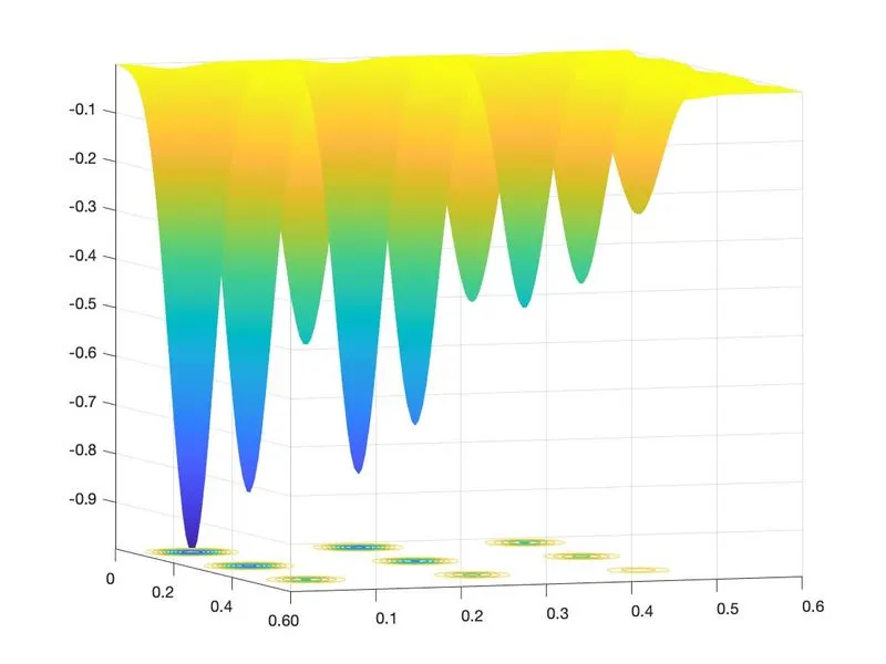
MAXIMA FOR THE FUNCTION STALAGMITE.M
PROGRAM FOR OPTIMIZATION USING GEOMETRIC ALGORITHM SHOWING MINIMA VALUE
clear all
close all
clc
% Defining our search space
x=linspace(0,0.6,150);
y=linspace(0,0.6,150);
num_cases=50;
%creating the two dimenasional mesh
[xx,yy]=meshgrid(x,y);
%evaluating the stalagmite function
for i=1:length(xx)
for j=1:length(yy);
input_vector(1)=xx(i,j);
input_vector(2)=yy(i,j);
f(i,j)=stalagmite(input_vector);
end
end
%study1-statistical behaviour
for i=1:num_cases
[inputs,fopt(i)]=ga(@stalagmite,2);
xopt(i)=inputs(1);
yopt(i)=inputs(2);
end
figure(1);
subplot(2,1,1);
hold on
surfc(x,y,f);
shading interp
plot3(xopt,yopt,fopt,'marker','o','markersize',5,'markerfacecolor','r');
title('unbound inputs');
subplot(2,1,2);
plot(fopt);
xlabel('iterations');
ylabel('function minimum');
tic
%study2-statistical behaviour-with upper and lower bounds
for i=1:num_cases
[inputs,fopt(i)]=ga(@stalagmite,2,[],[],[],[],[0;0],[1;1]);
xopt(i)=inputs(1);
yopt(i)=inputs(2);
end
study2_time=toc
figure(2);
subplot(2,1,1);
hold on
surfc(x,y,f);
shading interp
plot3(xopt,yopt,fopt,'marker','o','markersize',5,'markerfacecolor','r');
title('bound inputs')
subplot(2,1,2);
plot(fopt);
xlabel('iterations')
ylabel('function minimum')
%study3 increasing GA iteration
options=optimoptions('ga');
options=optimoptions(options,'Populationsize',170);
tic
for i=1:num_cases
[inputs,fopt(i)]=ga(@stalagmite,2,[],[],[],[],[0;0],[1;1],[],[],options);
xopt(i)=inputs(1);
yopt(i)=inputs(2);
end
study3_time=toc;
figure(3);
subplot(2,1,1);
hold on
surfc(x,y,f);
shading interp
plot3(xopt,yopt,fopt,'marker','o','markersize',5,'markerfacecolor','r');
title('bound inputs')
subplot(2,1,2);
plot(fopt);
xlabel('iterations')
ylabel('function minimum')
DETAILED EXPLANATION OF THE PROGRAM
-Giving command clear all,close all,clc
-defining the search space
x=linspace(0,0.6,150)
for the x coordinates
y=linspace(0,0.6,150)
for the y coordinates
-giving command num_cases=50
which means no.of times we repeat the value of the x and y we want repeatedly.
-creating the two dimensional mesh
[xx,yy]=meshgrid(x,y);
using the mesh grid command is used to create input matrix of the 2D surface grid from vector value x and y.
-evaluating stalagmite function
for i=1:length(xx)
Starting a "for loop' which will take the values of x coordinates of input matrix (xx,yy] from start to
end, which will be saved in the 'i'.
for j = 1: length (yy);
Starting a 'for loop' which will take the values of y coordinates of input matrix (xx,yy] from start to
end, which will be saved in the •j'.
end, which will be saved in the 'i'.
for j = 1: length (yy);
Starting a 'for loop' which will take the values of y coordinates of input matrix (xx,yy] from start to
end, which will be saved in the •j'.
- input_vec(1) = xx(i,j);
The input variable "input_vec(1)' holds the values of x,y coordinates of input matrix (xx,yy] of meshgrid
2D surface to plot the 3D surface along the x-axis.
The input variable "input_vec(1)' holds the values of x,y coordinates of input matrix (xx,yy] of meshgrid
2D surface to plot the 3D surface along the x-axis.
- input_vec(2) = yy(1,j);
The input variable "input_vec(2)' holds the values of x,y coordinates of input matrix (xx,yy] of meshgrid
-surface to plot the go surface along the y-axis.
The input variable "input_vec(2)' holds the values of x,y coordinates of input matrix (xx,yy] of meshgrid
-surface to plot the go surface along the y-axis.
- f(i,j) = F_stalagmite(input_vec);
The input variable f(i,j) holds the values of the stalagmite function which is used to create the 3D
surface by using a mathematical model.
The input variable f(i,j) holds the values of the stalagmite function which is used to create the 3D
surface by using a mathematical model.
-end
end of 'for loop' 1
end
end of 'for loop'2
-tic
To study the time required for the execution of the of Study-01 we are assigning the 'tic' command for
starting the timer which will evaluate the time required for Study-01.
starting the timer which will evaluate the time required for Study-01.
-% Study-01: Statistical Behaviour
Here we are evaluating the stalagmite function and finding the values of the minima for it.
Here we are evaluating the stalagmite function and finding the values of the minima for it.
- for 1 = 1:num_cases
Starting 'for loop' which will take values from 1 to 50 (num_cases)
Starting 'for loop' which will take values from 1 to 50 (num_cases)
-[inputs, fopt(1)] = ga(@stalagmite, 2);
Entering the syntax of 'ga' under input variable (inputs, fopt(1)] 'ga' will evaluate the function
'stalagmite' which consists of two variables.
Entering the syntax of 'ga' under input variable (inputs, fopt(1)] 'ga' will evaluate the function
'stalagmite' which consists of two variables.
-x0pt(i) = inputs(1) ;
The optimum value of × is saved under the input variable 'xopt(i)* for every single loop which is taken from the input variable
"inputs of 'ga' syntax.
The optimum value of × is saved under the input variable 'xopt(i)* for every single loop which is taken from the input variable
"inputs of 'ga' syntax.
-y0pt(i) = inputs(2) ;
The optimum value of y is saved under the input variable 'yopt(i)* for every single loop which is taken from the input variable
"inputs of 'ga' syntax.
The optimum value of y is saved under the input variable 'yopt(i)* for every single loop which is taken from the input variable
"inputs of 'ga' syntax.
-end
end of for loop
-figure(1)
-subplot (2,1,1)
Figure(1) is saved under the command "subplot' which consists of three numeric digits. The main objective of the"subplot command to represent the two or more than two figures in the same frame. The very first digit in the command represents the number of rows, second digit represents the number of columns the third digit represents the number of sub-figure.
- xlabel(X-Axis)
- ylabel("Y-Axis*)
Figure(1) is saved under the command "subplot' which consists of three numeric digits. The main objective of the"subplot command to represent the two or more than two figures in the same frame. The very first digit in the command represents the number of rows, second digit represents the number of columns the third digit represents the number of sub-figure.
- xlabel(X-Axis)
- ylabel("Y-Axis*)
zlabel('zaxis')
Labeling X, Yand Z axis of the plot.
- hold on
-surfc(x,y, f)
objective of the conmand "surfc(x,y,f)* is to plot the function plot *f" on the Z-axis on the 20 arid defined by the x and y coordinates. This figure of "surfe' conmand is first sub-figure under the 'subplot command.
-shading interp
shading interp varies the color in each line segment and face by interpolating the colormap index or true color value across the line of face.
Labeling X, Yand Z axis of the plot.
- hold on
-surfc(x,y, f)
objective of the conmand "surfc(x,y,f)* is to plot the function plot *f" on the Z-axis on the 20 arid defined by the x and y coordinates. This figure of "surfe' conmand is first sub-figure under the 'subplot command.
-shading interp
shading interp varies the color in each line segment and face by interpolating the colormap index or true color value across the line of face.
- plot3(xopt, yopt, -fopt, "marker', 'o' , "markersize',5, "sarkerfacecolor', 'r*)
Commanding the 'plot3' for plotting optimum values of x,y and f of specified input credentials.
Commanding the 'plot3' for plotting optimum values of x,y and f of specified input credentials.
- title('unbounded inputs*)
Title of the plot 'unbound inputs'
Title of the plot 'unbound inputs'
- subplot (2,1,2)
- plot(-fopt)
Plotting the second sub-figure of the 'subplot' command which will plot the values of
for minia
- xlabel("Iterations*)
-ylabel("Function minimun*)
Labeling the x and y axises of the second sub-figure..
- study01_time = toc
End of timer for the evaluation of the time required for the execution for Study-01.
Plotting the second sub-figure of the 'subplot' command which will plot the values of
for minia
- xlabel("Iterations*)
-ylabel("Function minimun*)
Labeling the x and y axises of the second sub-figure..
- study01_time = toc
End of timer for the evaluation of the time required for the execution for Study-01.
-tic
-study-02: statistical behaviour with upper and lower bound
- for 1 = 1: num_cases
[inputs, fopt(i)] = ga(@stalagmite, 2, [], [], [], [], (0: 0], [1: 1) ) ;
The selection of the points for the evaluation is very random and unspecified therefore to overcome this we have to put the upper and lower bounds on the points under consideration. [0:0] defines the lower bounds and [1:1] defines the upper bounds. Now it means for every single run
the values for the points of section will range between (0:0] to (1:1).
- xopt(i) = inputs (1) ;
- yopt(i) = inputs (2);
[inputs, fopt(i)] = ga(@stalagmite, 2, [], [], [], [], (0: 0], [1: 1) ) ;
The selection of the points for the evaluation is very random and unspecified therefore to overcome this we have to put the upper and lower bounds on the points under consideration. [0:0] defines the lower bounds and [1:1] defines the upper bounds. Now it means for every single run
the values for the points of section will range between (0:0] to (1:1).
- xopt(i) = inputs (1) ;
- yopt(i) = inputs (2);
-end
end of for loop
-study02_time=toc
-figure(2)
figure command in order to save the separate figure by the name figure 2
-subplot (2,1,1)
- xlabel(X-Axis)
- ylabel("Y-Axis*)
- xlabel(X-Axis)
- ylabel("Y-Axis*)
-zlabel('zaxis')
- hold on
-surfc(x,y, f)
-shading interp
- hold on
-surfc(x,y, f)
-shading interp
- plot3(xopt, yopt, -fopt, 'marker', 'o' , "markersize',5, "sarkerfacecolor', 'r')
- title('bounded inputs*)
- subplot (2,1,2)
- plot(-fopt)
- xlabel("Iterations'')
-ylabel("Function minimun'')
- xlabel("Iterations'')
-ylabel("Function minimun'')
-study03:bounded with modified population size
options=optimoptions('ga');
options=optimoptions(options,'Populationsize',170);
Startup options instruct matlab to perform certain operations when you start the program.
Startup options also are called command flags or command-line switches. When you start at the operating system
prompt, specify the options as arguments to the matlab command.
The population size is stated in the command. Here the polulaton size means the total number of values
taken into consideration fk the study i.e. 180 so that larger the size more easier it becomes for'ga' to
compare and study and evaluate the minima, the only drawback is this process takes a comparatively more time.
Startup options also are called command flags or command-line switches. When you start at the operating system
prompt, specify the options as arguments to the matlab command.
The population size is stated in the command. Here the polulaton size means the total number of values
taken into consideration fk the study i.e. 180 so that larger the size more easier it becomes for'ga' to
compare and study and evaluate the minima, the only drawback is this process takes a comparatively more time.
-tic
-for i=1:num_cases
-[inputs,fopt(i)]=ga(@stalagmite,2,[],[],[],[],[0;0],[1;1],[],[],options);
-xopt(i)=inputs(1);
-yopt(i)=inputs(2);
-end
-study3_time=toc;
-figure(3);
-subplot(2,1,1);
-hold on
-surfc(x,y,f);
-shading interp
-plot3(xopt,yopt,fopt,'marker','o','markersize',5,'markerfacecolor','r');
title('bound inputs')
-subplot(2,1,2);
-plot(-fopt);
-xlabel('iterations')
-ylabel('function minimum')
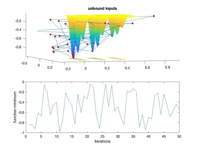
FIGURE1 FOR STUDY 1
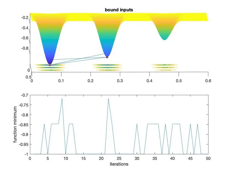
FIGURE2 FOR STUDY 2
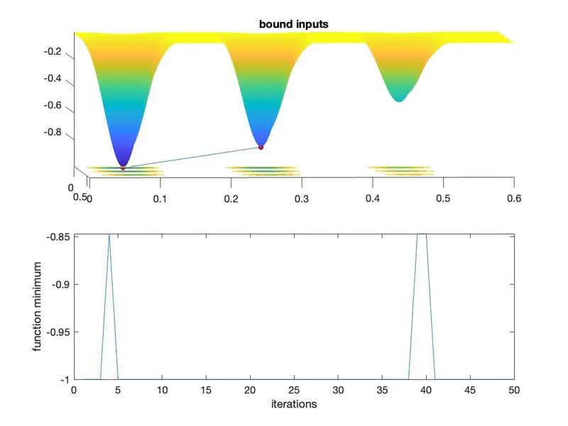
FIGURE3 FOR STUDY 3
PROGRAM03: FUNCTION PROGRAM FOR STALAGMITE
function [f]=stalagmite(input_vector)
x=input_vector(1)
y=input_vector(2)
f1=(sin(5.1*pi*x+0.5))^6
f2=(sin(5.1*pi*y+0.5))^6
f3=exp(-4*log(2)*(x-0.0667)^2/0.64);
f4=exp(-4*log(2)*(y-0.0667)^2/0.64);
f=-(f1*f2*f3*f4);
end