Project 2 - Rankine cycle Simulator

OBJECTIVE:Write a matlab code on Rankine Cycle simulator and plot H-S & T-S Diagram

PROBLEM STATEMENT:
• Create a rankine cycle simulator using MATLAB
Our code should calculate the state points of the rankine cycle based on user inputs.
then plot the corresponding T-S & H-S plots for the given set of inputs. Title and axes labels are a must, while legends could be used
if necessary.
the presentation of our code will be taken into considerations while grading. Labelling section of our code using comments is
appreciated
Attach a report explaining the working of a rankine cycle simulator and also research done by us.

Contents expected in the report:
Step wise explaination of our code
Mention the errors faced while programming
Steps taken to overcome those errors
Screenshots showing errors thrown in command window.

Required inputs:
Turbine inlet temperature = 400 degree celcius
Turbine Inlet Pressure = 30 bars
Turbine outlet pressure = Condenser inlet pressure = 0.05 bars
Calculate the following-
• Net work output
Back work ratio
THEORY & INTRODUCTION:-
The Rankine Cycle is one of many thermodynamic cycles that is used to produce mechanical work. This cycle in particular is used to predict
the work produced by a steam turbine system in a heat engine. Heat engines are commenly found in things like trains and air conditioners.
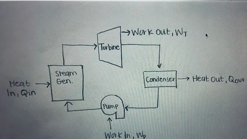
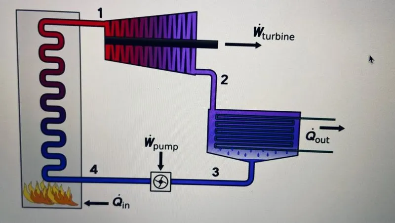
The rankine cycle consist of four different components are-
1. Steam generator :- Turns the fluid at room temperature and pressure, to vapour or steam at an extremely high temperature, usualy
turmed "Superheated Vapor.
2. Turbine :- The pressure is increase, resulting in a drop in temperature and producing mechanical work that leaves the system tobe used.
3. Condenser:- Operates at a constant pressure where heat is released into the enviornment, compressing the state of the fluid back down
to a liquid gas mixture, that is mostly liquid. This state is otherwise known as "Saturated liquid
4. Pump:- Pressured the saturated liquid back up to the pressure of the turbine by bringing work back into the system, turning to a highly
pressurized liquid which is usually reffered to as a "Compressed Liquid
Finally, the fluid goes back through the steam generator at constant pressure to return to a superheated vapor.

In order to easily analyse the Rankine Cycle, there are many idealization that engineers commenly make, so that the system can be
understood in ideal situations. Additionally, there are some things throughout the cycle analysis that we will consider tobe "ideal' meaning
they work without any imperfections. Engineers tends to make these assumptions when analysing systems, in order to have an accurate
representationof what is going on. But the fact is that nothing ever works out exactly how we expect or calculate and does not act the same
way every time. This is especially true in the analysis of the Rankine Cycle. The reason that we say we are an;lysing a "Simple, Ideal Rankine
Cycle" is because it is exactly that; simplified and ideal. In reality there are dozens of things that would have tobe accounted for to get an
exact calculation, but they will be ignored for now in order to get a fundamental understanding of the cycle itself.
The concept and vocabulary needed to consider the system ideal are-
Adiabatic:- Does not loose heat
Isentropic:- Adiabatic and reversible or no change in entropy. Used when analysing the turbine and pump
Isobaric:- Constant pressure; considered when analysing the steam generator and condenser
Steady state :- the state of the fluid does not change with time
Steady flow :- that the mass of fluid flowing through the system is constant everywhere.
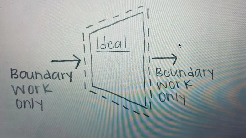
Boundary work : - Only consider changes that happens across the boundary of each component. There are other things that go on inside
each component, but they are neglected for simplicity, since the final result would not be that different if they are included.

Compressed Liquid:A liquid that has been completely pressurised.

Pressure(P) :- One of the most important proparties, because it is usually given, allowing us to easily look up other proparty in our state
Tables, and gives us an easy gage for where we are as we travel through the cycle.

Temperature(T) :- Is not always necessary to record but is used to give you of an idea of where you are in the cycle, and a gage that is easily
understood. It is also listenin the state table, so it is sometimes useful to look up other proparties.

Entropy(S) :- An abstract concept used to represent the changes that occur to heat due to temperature.

Enthaly(h) :- Measure of the internal energy within a system. Each component analysed will be considered a 'system', allowing us to find an
enthalpy value for each. This is essentially how the heat transfers through each of the components, and how we keep track of it's increase
and decreases. Enthalpy is the proparty we will used to calculate work at the end according to the first law of thermodynamics.

Specific Volume (v):- Calcualted based on the volume of fluid per unit mass (different from total voume, which is unnecessary) and is used
in this cycle to calculate the enthalpy out of the pump.

Quality(x):- Measure of fluids liquid-gas mixture. If the fluid is in a superheated vapor state, or compressed liquid state it will not have a
quality. Otherwise, it is a mixture of liquid and gas and the value will range from O to 1, O being a saturated liquid (still unpressurized but they
close to the pressure limit) and 1 being a saturated vapor (steam, on the verge of being superheated).

STEP BY STEP CODE EXPLAINATION:=
1. First of all display the all four points which are on the rankine cycle (display command is used only for temperory reading and not save
in memor).
2. described pressure and temperature values by user defined.
3. find out the value of enthalpy(h1) and entropy(s1) from pressure and temperature from XSteam library in mattab,
4. XSteam library is nothing but the steam table, which is put in the same directory where matlab program saved.
5. Find out all the points of inlet & outlet of turbine, condenser, pump and boiler.
6. Also find out the work done of pump and turbine
7. At state1 & 3 p3-p2 & p4=p1.
8. Find out net workdone, heat supplied, heat rejected, efficiency & specific steam consumption.
9. finally plot the H-S and T-S plots.
10. Link all the points i.e. 1-2-3-4-1.
11. gives the legend, title, label & label.
12. output the values of P, T, H, S for each state respectively.

MAIN CODE:

% Renkine Cycle Simulator

clear all

close all

clc

disp('RANKINE CYCLE SIMULATOR')

disp('1-2 is isentropic expension in turbine')

disp('2-3 is constant pressure heat rejection in condensor')

disp('3-4 is isentropic compression in pump')

disp('4-1 is constant pressure heat addition in boiler')

p1=input('enter the pressure at inlet of turbine(in bar)= ');

t1=input('enter the temprature at inlet of turbine(in degree celcius)= ');

p2=input('enter the pressure at the inlet of condenser(in bar)= ');

%Steam Condition at the inlet of turbine

h1=XSteam('h_pt',p1,t1);

s1=XSteam('s_pt',p1,t1);

%Steam condition at the outlet of turbine

sg2=XSteam('sV_P',p2);

sf2=XSteam('sL_p',p2);

sfg2=sg2-sf2;

x2=(s1-sf2)/sfg2;

s2=sf2+x2*sfg2;

hf2=XSteam('hL_p',p2);

hg2=XSteam('hv_p',p2);

hfg2=hg2-hf2;

h2=hf2+x2*hfg2;

t2=XSteam('Tsat_p',p2);

%Workdone by turbine

W_T=h1-h2;

%Steam condition at the outlet of condensor

p3=p2;

t3=XSteam('Tsat_p',p2);

h3=XSteam('hL_p',p2);

s3=XSteam('sL_p',p2);

vf=XSteam('vL_p',p2);

t2=t3;

%Calculate the pump work

W_P=vf*(p1-p2)*100;

%Steam condition at the state 4

p4=p1;

h4=W_P+h3;

s4=s3;

t4=XSteam('T_ph',p4,h4);

%Net Workdone

W_net=W_T-W_P;

%Heat Supplied

Q_s=h1-h4;

%Heat Rejected

Q_r=h2-h3;

%Efficiency

efficiency=(W_net/Q_s);

%specific steam consumption

SSC=3600/W_net;

tf_sat=XSteam('Tsat_p',p1);

sf_sat=XSteam('sL_p',p1);

hf_sat=XSteam('hL_p',p1);

sg_sat=XSteam('sV_p',p1);

hg_sat=XSteam('hV_p',p1);

%Plotting T-S Diagram

hold on

%for plotting saturation curve

tsat1=linspace(0,374,1000);

for i=1:length(tsat1)

ss1(i)=XSteam('sL_T',tsat1(i));

end

for j=1:length(tsat1)

ss2(j)=XSteam('sV_T',tsat1(j));

end

plot(ss1,tsat1,'b');

plot(ss2,tsat1,'r');

%for saturation temprature at p1

temp=XSteam('Tsat_p',p1);

t=linspace(t4,temp,30);

for i=1:length(t);

S(i)=XSteam('s_pt',p1,t(i));

hold on

end

t0=linspace(temp,t1,300);

for i=1:length(t0)

s0=XSteam('s_pt',p1,t0(i));

end

%for plotting turbine work

plot([s1 s2],[t1 t2],'g');

%for heat rejection in condensor

plot([s2 s3],[t2 t3],'b');

%for pump work

plot([s3 s4],[t3 t4],'r');

%plotting curve line (constant pressure line in wet region) from outlet of

%the pump to the point from where the phase change start

plot(S,t,'Y');

%Plotting the phase change region

plot([sf_sat sg_sat],[tf_sat tf_sat],'Y');

%plotting the curved constant pressure line from where the phase change

%ends to the super heated point

plot(s0,t0,'y');

legend('Saturation Curve L','Saturation Curve V','Turbine','Condenser','Pump','Boiler','l');

title('T-S Diagram');

xlabel('Entropy');

ylabel('Temprature');

%plotting H-S Diagram

figure(2);

hold on

%for plotting the saturation curve

tsat1=linspace(0,374,1000);

for i=1:length(tsat1)

hh1(i)=XSteam('hL_T',tsat1(i))

end

for j=1:length(tsat1)

hh2(j)=XSteam('hV_T',tsat1(j));

end

plot(ss1,hh1,'b');

plot(ss2,hh2,'r');

%for plotting turbine

plot([s1 s2],[h1 h2],'g');

%for plotting condensor

plot([s2 s3],[h2 h3],'b');

%for plotting pump

plot([s3 s4],[h3 h4],'r');

s=linspace(s3,s1,1000);

for i=1:length(s)

h(i)=XSteam('h_ps',p1,s(i));

end

%for plotting boiler

plot([s4 s1],[h4 h1],'y');

plot(s,h,'y');

legend('Saturation Curve L','Saturation Curve V','Turbine','Condenser','Pump','Boiler','l');

title('H-S Diagram');

xlabel('Entropy');

ylabel('Enthalpy');

%back work ratio

BWR=-(W_P/W_T);

%OUTPUT

%At State-1

fprintf('AT state point-1:rn')

fprintf('p1 is:%f Barrn',p1)

fprintf('T1 is :%f Deg Celciusrn',t1)

fprintf('H1 is :%f KJ/KGrn',h1)

fprintf('S1 is :%f KJ/KGKrn',s1)

%At State-2

fprintf('AT state point-2:rn')

fprintf('p2 is:%f Barrn',p2)

fprintf('T2 is :%f Deg Celciusrn',t2)

fprintf('H2 is :%f KJ/KGrn',h2)

fprintf('S2 is :%f KJ/KGKrn',s2)

fprintf('X is :%f rn',x2)

%At State-3

fprintf('AT state point-3:rn')

fprintf('p3 is:%f Barrn',p3)

fprintf('T3 is :%f Deg Celciusrn',t3)

fprintf('H3 is :%f KJ/KGrn',h3)

fprintf('S3 is :%f KJ/KGKrn',s3)

%At Point-4

fprintf('AT state point-4:rn')

fprintf('p4 is:%f Barrn',p4)

fprintf('T4 is :%f Deg Celciusrn',t4)

fprintf('H4 is :%f KJ/KGrn',h4)

fprintf('S4 is :%f KJ/KGKrn',s4)

% Calculations

fprintf ('Work done by Turbine : %f KJ/Kgrn',W_T)

fprintf ('Work done by pump : %f KJ/Kgrn',W_P)

fprintf('Heat added in the boiler : %f KJ/Kgrn',Q_s)

fprintf('Heat rejected in the condenser : %f KJ/Kgrn',Q_r)

fprintf('Thermal efficiency is : %f %%rn' ,efficiency*100)

fprintf('Species Steam Consumption : %f KJ/Kwhrn',SSC)

fprintf('Back Work Ratio :%f %%rn' ,BWR*100)

OUTPUT PLOTS:

TEMPRATURE VS ENTROPY PLOT:

Above diagram shows the temperature vs entropy values. From point 1-2, as temperature increases, entropy also increases and vice versa.
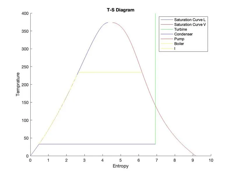
From point 2-3 temperature remains constant but entropy increases contineously due to the turbine work as shown in Azure. Then
temperature increases upto critical point and then decreases at constant entropy and reducing temperature. From 4-1 temperature remain
constant at low range and reach to the condenser through pump.
From point 3-4 temperature decreases because of cooling effect through heat exchanger i.e. fan. Here, turbine gives positive work while
pump gives negative work and according to that entropy increases and decreases respectively.

ENTROPY VS ENTHALPY PLOT:

As we know that, entropy is directly proportional to the enthalpy, which is clearly prooved from above diagram. At very small change of
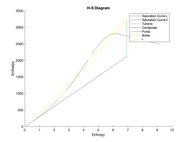
entropy, enthalpy change widely as shown in the above figure. At turbine work is produced and that's why enthalpy increases at constant
entropy and thereafter this same cycle comes back with same rate of change. Turbine produces work at constant entropy while condenser
produces work directity from entropy and enthalpy change. the rate of change of boiler is nearly same from start to end cycle.

OUTPUT:

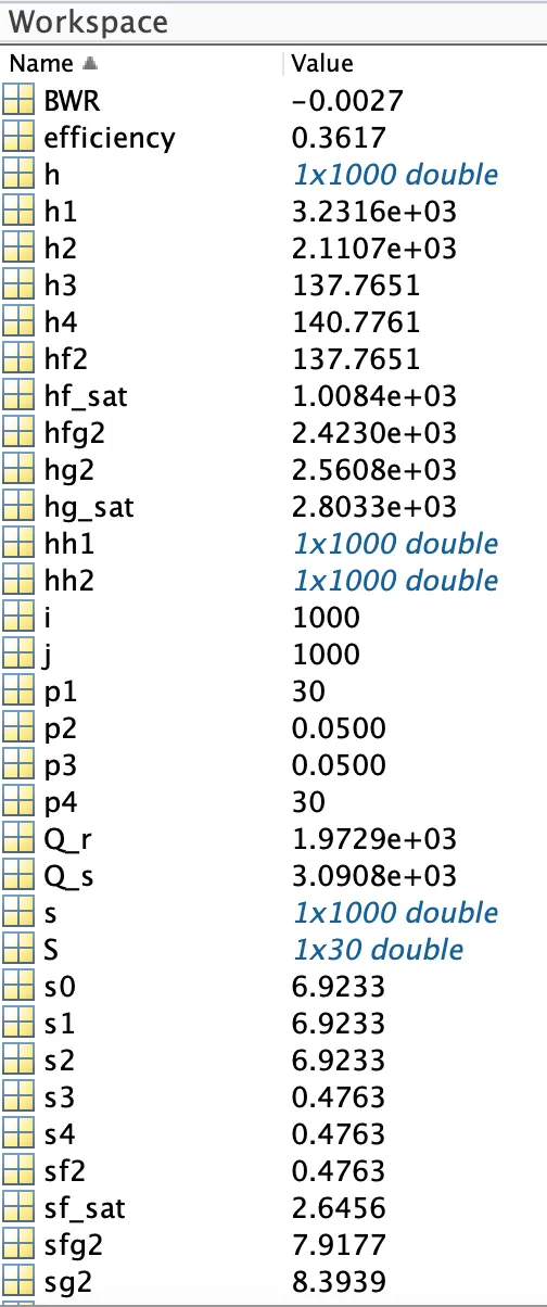
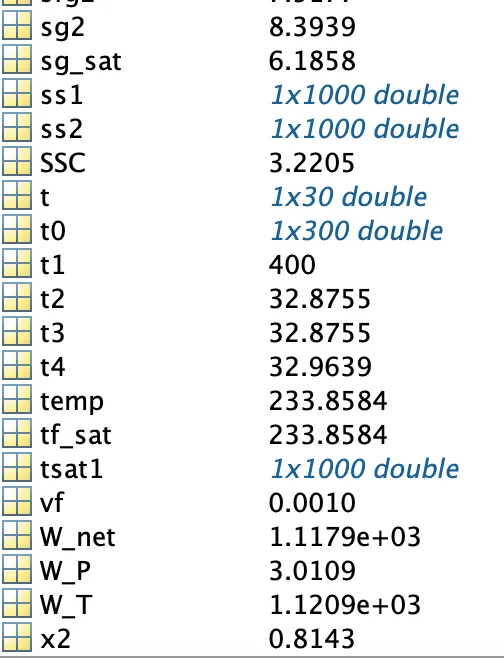
AT state point-1:rnp1 is:30.000000 BarrnT1 is :400.000000 Deg CelciusrnH1 is :3231.571027 KJ/KGrnS1 is :6.923259 KJ/KGKrnAT

state point-2:rnp2 is:0.050000 BarrnT2 is :32.875490 Deg CelciusrnH2 is :2110.708212 KJ/KGrnS2 is :6.923259 KJ/KGKrnX is :0.814256 rnAT

state point-3:rnp3 is:0.050000 BarrnT3 is :32.875490 Deg CelciusrnH3 is :137.765119 KJ/KGrnS3 is :0.476254 KJ/KGKrnAT

state point-4:rnp4 is:30.000000 BarrnT4 is :32.963884 Deg CelciusrnH4 is :140.776056 KJ/KGrnS4 is :0.476254 KJ/KGKrn

Work done by Turbine : 1120.862815 KJ/Kgrn

Work done by pump : 3.010937 KJ/Kgrn

Heat added in the boiler : 3090.794971 KJ/Kgrn

Heat rejected in the condenser : 1972.943093 KJ/Kgrn

Thermal efficiency is : 36.167131

Steam Consumption : 3.220462 KJ/Kwhrn

Back Work Ratio :-0.268627 %rn>>

Back Work Ratio:
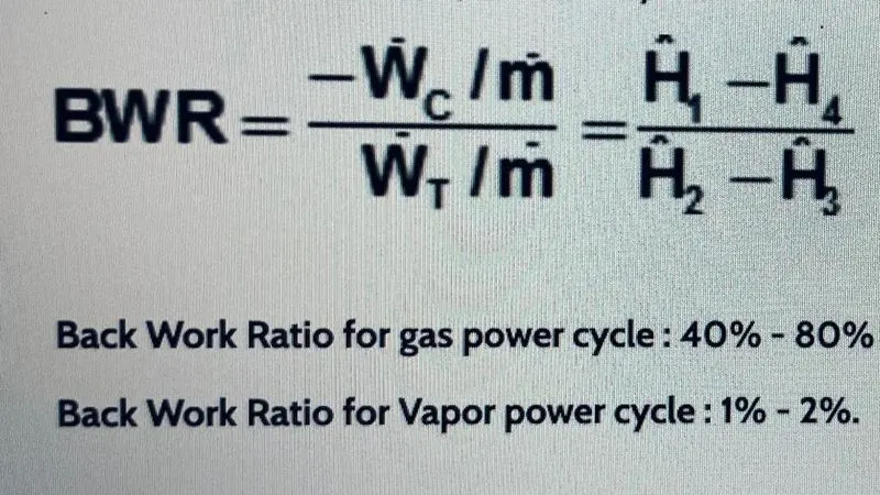
The fraction of the work produced by the turbine that is consumed by the pump.

ERROR AND REMEDIES:-
1.
Cannot find an exact (case-sensitive) match for 'Xsteam'
The closest match is: XSteam in F:(MATLAB Challenge\ Seventh Week\XSteam.m
Error in rankine cycle (line 18)
h1= Xsteam ('h_pt', pl, t1)
This error occurs due to incorrect name of saved file. As we know that, Matlab is a case sensitive, and if there have not matches a single
words, it popup the error and thrown in the command window. For rectifying this error we need to make confirm written name in Matlab
and file saving name in the same directory must be same otherwise, it showing same error.
2.
Relat
>› rankinecycle
Error: File: rankine cycle.m Line: 170 Column: 8
Character vector is not terminated properly.
This error occurs de to absent of parenthesis on either side. To solve this error we need to make confirm that, parenthesis must be on both
he pronar manner otherwise, it popup error in command window. This is due to MATIAR is a scientific programming language and it works on matrix.

CONCLUSION:

1. When work produced through turbine and work consumed through condener, in both the casses entropy change but temperature
remains constant (from T-S diagram).
2. When fluid is enters through the heat exchanger i.e. fan, only temperature decreases, entropy remains constant (from T-S diagram).
3. After turbine work temperature rise upto critical point and then goes down.

In this way I write a detailed code in MATLAB, plot the T-S & H-S diagram as shown above. Also I found some errors which are described
above. Finally, I concluded some important points are described above.

THANKS

RUMMAN KHAN.