Week 4.1 - Genetic Algorithm

Aim- Writing the code in MATLAB to optimize the stalagmite function and also for finding the global maxima of the function.

Objective – To know how GA (Genetic Algorithm) works. The concept behind it and how to get the Local/Global-minima/maxima.

Equations- f(x,y) = (f1.x)*(f1.y)*(f2.x)*(f2.y)

F1.x = [sin(5.1*pi*x+0.5)]⁶

F1.y= [sin(5.1*pi*y+0.5)]⁶

F2.x= exp[-4ln(2)*((x-0.0667)² /(0.64))]

F2.y= exp[-4ln(2)*((y-0.0667)² /(0.64))]

Inputs provided –

x = linspace (0,0.6,150)

y = linspace (0,0.6,150)

GENETIC ALGORITHM –

Is a search-based optimization technique based on the principles of Genetics and Natural Selection. It is frequently used to find optimal or near-optimal to difficult problems which otherwise would take a lifetime to solve.

Shortly, it is one of the machine learning algorithms that is used to get optimized results.

It is widely used today in Business, scientific & engineering circles.

This algorithm reflects the process of natural selection where the fittest individuals are selected for reproduction in order to produce offspring of the next generation.

Now just understand what is optimisation.

Optimisation - It is a decision making process, it helps to find best results under a set of prioritized criteria or constraints. It is a procedure which is executed iteratively by comparing various solutions till an optimum or a satisfactory solution is found. It works on following three main steps.

1. Selection
2. Crossover

Selection – A no of individuals is selected from the population in the mating pool, based on the previously calculated fitness value, the best individuals base on the threshold are selected after that we will end selecting a subset of the population in the mating pool.

Crossover – Crossover in GA generates a new generation same as the natural mutation, by mutating the old generation parents, the new generation offspring comes by carrying genes from both parents. The amount of genes carried from each parent is random.

Mutation - For each offspring select some genes and changes its value, mutation prevents the

solution from falling into a local minima.

Stopping Criteria –

1. Generations (Iterations) – the algorithm is stops when the given iterations are completed.
2. Time limit – Time taken by the algorithm is depends on the complexity of the equations

Which is also measured in the 3 studied performed.

3. Fitness limit – The algorithm stops when the value of the fitness function for the best point in the current population is reached to the optimized value or (fitness limit)

Program codes explanation –

1. clear all – It is used to clear all the variables inserted from the work space.
2. Close all – It is used to clear or close opened figures or images.
3. Clc – It is used to command window.

Creating one Dimensional array with random nos.

X & Y with linspace command

Then converted that to 2 dimensional array with meshgrid command

Meshgrid is ued to multiply the arrays, with this one dimensional array is converted into 2-dimensional array.

After this we are using double for loop for the 2-dimensional array we just created which will give us the random set of values that can be used in a stalagmite function to get the optimum solution.

STALAGMITE – Stalagmite structures are formed from the curved floor that point upward.

Stalagmite & stalactite function are mathematical functions which represents shapes similar to that of the stalagmite & stalactite function.

Syntax- ga(fun,nvars) finds a local unconstrained minimum, x, to the objective function, fun. nvars is the dimension (number of design variables) of fun.

x = ga(fun,nvars,A,b,Aeq,beq,lb,ub) defines a set of lower and upper bounds on the design variables, x, so that a solution is found in the range lb ≤ x ≤ ub. (Set Aeq=[] and beq=[] if no linear equalities exist.)

x = ga(fun,nvars,A,b,Aeq,beq,lb,ub,nonlcon,options) minimizes with the default optimization parameters replaced by values in options. (Set nonlcon=[] if no nonlinear constraints exist.) Create options using optimoptions.

For Plotting more than one graph we will create figures following with numbers

Like figure(1), figure(2)

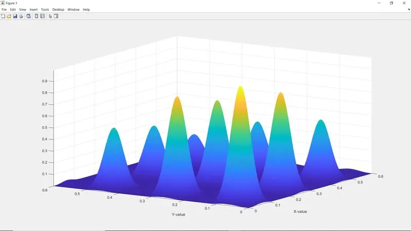
Plotted the 1^st graph and the stalagmite function for random numbers it is observed that our result value is changing after every run of program.

Hence we done the coding to know the statistical behaviour of the plot and the results how it changes. For this num_cases is the function used to run the code for 50 times and those 50 values are observed to know the statistical behaviour of the genetic algorithm.

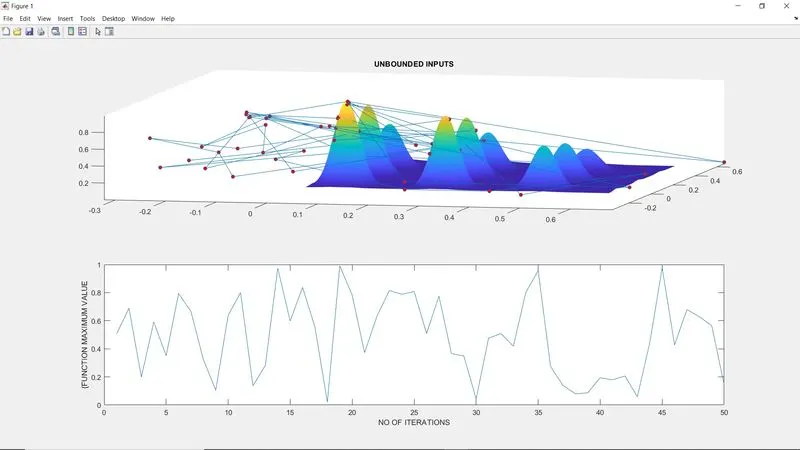
In this we used subplot command to compare graphs subplot command is used to get more than one graph in one figure window. And also modified the for loop with x-values and y-values. Also in this study we used the plot3 command which gives the x, y and f (ie.result) to get perfect comparison. We used the tic and toc command to know how much the study will take.

After observing the graph it is noticed that the stalagmite function values and the result values are not as expected as it is random sampling. And the values are sprayed all over the graph over the range.

Time taken by study 1 – 2.2866 sec.

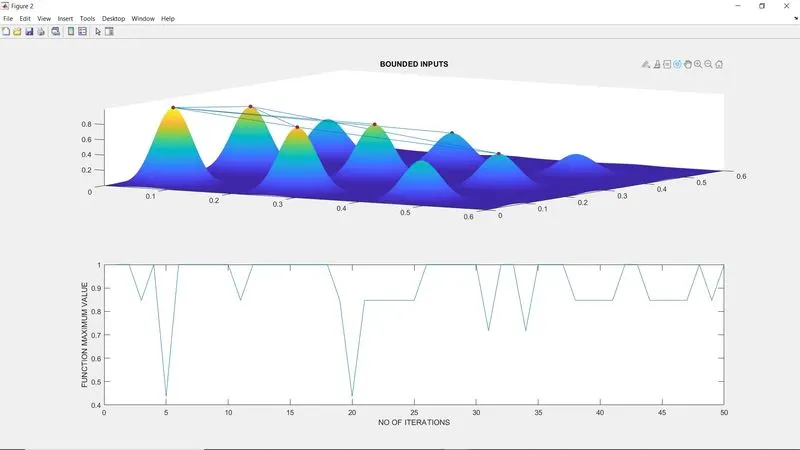
In study no 2 we set up the bounds (limits) upper bound and lower bound. And run the code

Now in this our results shows the answers In the limits provided and also précised from the last one

Also the graph looks neat and aligned. But still the results are precise not accurate.

If we have smaller population size then we are only able to get local minima, for this we have to increase the population size.

Time taken by study 2 – 3.4453 sec.

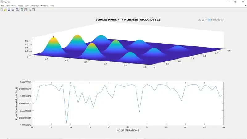
Hence in study no 3 we increased the initial size of the population by 200.

And as the result of this we got the global maxima.

Time taken by study 1 – 19.94 sec.

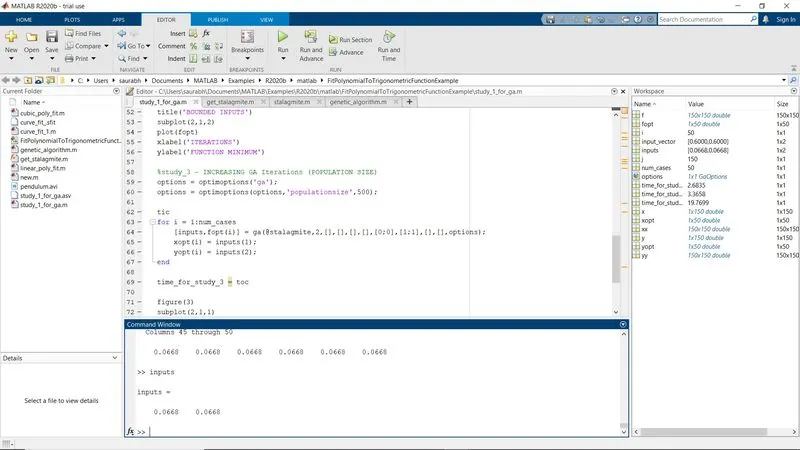
The global maxima is at point (x = 0.0668, y= 0.0668)

Conclusion – Understood the logic of GA and stalagmite function

clear all
close all
clc
%Defining Search Space
%linspace creates random values from 0 to 0.6, 150 individual values
x = linspace (0, 0.6, 150); 
y = linspace (0, 0.6, 150);
%no of Iterations = num_cases
num_cases = 50;
%Creating 2Dimensional Mesh
[xx yy] = meshgrid(x, y);
%Evaluating the stalagmite Function
for i = 1:length (xx);
    for j = 1:length (yy);
        input_vector(1)=xx(i, j);
        input_vector(2)=yy(i, j);
        f(i, j) = stalagmite(input_vector);
    end
end
figure(1)
%surfc creates the 3D-plot with creating surface of coordinates 
surfc (xx,yy, -f)
%name given to x- axis (x-value)
xlabel('X-value')
%name given to y- axis (y-value)
ylabel('Y-value')
%title given to the graph
title('RANDOM GA')
%shading interp creates the clean smooth plot without grid lines 
shading interp
[inputs, fval] = ga(@stalagmite, 2);

%Study_1 - Statastical Behavior
tic
for i = 1:num_cases
    [inputs, fopt(i)] = ga(@stalagmite, 2);
    xopt (i) = inputs(1);
    yopt (i) = inputs(2);
end
time_for_study_1 = toc
figure (2)
%subplot it can divide the figure window into 1x2,2x2 shape 
%subplot [(no of rows),(no of column),(figure no.)]
subplot (2, 1, 1)
hold on
surfc (x,y,-f)
shading interp
%plot3 contains x,y,and result plotted by x&y
plot3(xopt,yopt,-fopt,'marker','o','markersize',5,'markerfacecolor','r')
%title given to the graph
title('UNBOUNDED INPUTS')
subplot(2,1,2)
plot(-fopt)
%name given to x- axis (no of iterations)
xlabel('NO OF ITERATIONS')
%name given to y- axis (function maximum value)
ylabel('{FUNCTION MAXIMUM VALUE')

%study_2 - statistical behavior with upper and lower bounds
tic
for i = 1:num_cases
    [inputs, fopt(i)] = ga(@stalagmite,2,[],[],[],[],[0;0],[1;1])
    xopt(i) = inputs(1);
    yopt(i) = inputs(2);
end
time_for_study_2 = toc

figure(3)
subplot(2,1,1)
hold on
surfc(x,y,-f)
shading interp
plot3(xopt,yopt,-fopt,'marker','o','markersize',5,'markerfacecolor','r')
%title given to the graph
title('BOUNDED INPUTS')
subplot(2,1,2)
plot(-fopt)
%name given to x- axis (no of iterations)
xlabel('NO OF ITERATIONS')
%name given to y- axis (function maximum value)
ylabel('FUNCTION MAXIMUM VALUE')

%study_3 - INCREASING GA Iterations (POPULATION SIZE)
options = optimoptions('ga');
options = optimoptions(options,'populationsize',500);

tic
for i = 1:num_cases
    [inputs,fopt(i)] = ga(@stalagmite,2,[],[],[],[],[0;0],[1;1],[],[],options);
    xopt(i) = inputs(1);
    yopt(i) = inputs(2);
end

time_for_study_3 = toc

figure(4)
subplot(2,1,1)
hold on
surfc(x,y,-f)
shading interp
plot3 (xopt,yopt,-fopt,'marker','o','markersize',5,'markerfacecolor','r')
%title given to the graph
title('BOUNDED INPUTS WITH INCREASED POPULATION SIZE')
subplot(2,1,2)
plot (-fopt)
%name given to x- axis (no of iterations)
xlabel('NO OF ITERATIONS')
%name given to y- axis (function maximum value)
ylabel('FUNCTION MAXIMUM VALUE')