Project 2 - Rankine cycle Simulator

Aim –

1. To develop a simple program that calculates the state points of Rankine Cycle.
2. By adding the thermodynamic relations creating a simulator for Rankine cycle.
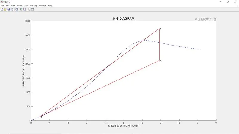
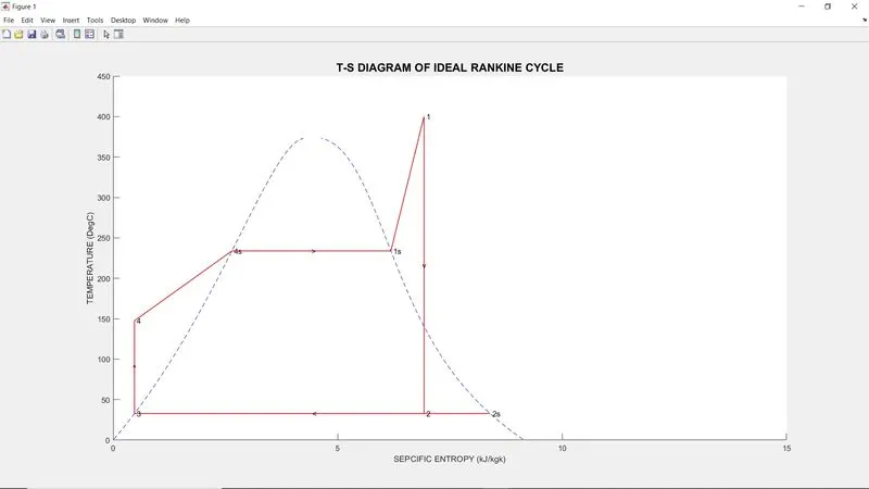
3. And plotting the Outputs in graphs with T-S and H-S plots.

Objective - To understand how to simulate the data in MATLAB, Extracting the data.

Background Knowledge – There are different GAS CYCLES were in use according to their purpose and fuel used.

Two primary classes of thermodynamic cycles are POWER CYCLES and HEAT PUMP CYCLES.

Power cycles are cycles which convert some heat input into a mechanical work output.

While, Heat pump cycles transfer heat from low to high temperatures by using mechanical work as input.

RANKINE CYCLE – It is an idealised thermodynamic cycle describing the process by which certain heat engines, such as steam turbines or reciprocating steam engines, allow mechanical work to be extracted from a fluid as it moves between a heat source and heat sink.

The Rankine cycle is named after William Jhon Macquom Rankine, a Scottish polymath professor at Glasgow University.

The ideal Rankine cycle does not involve any internal irreversibility and consist of following 4 Processes-

1. 1-2 – Isentropic Compression in Pump.
2. 2-3 – Constant Pressure Heat Addition in Boiler.
3. 3-4 –Isentropic Expansion in Turbine.
4. 4-1 –Constant Pressure Heat Rejection in Condenser.

The Thermal Efficiency of the Rankine Cycle is determined from –

Ƞth = (W)net /(Q)in

= 1 – (((Q)out)/((Q)in))

Where, (W)net = (Q)in – (Q)out

= (W)turbine output – (W)pump input

PROCESS EXPLAINATION –

Process 1-2 – The working fluid is pumped from low to high pressure, As the fluid is liquid at this stage, the pump requires little input energy.

Process 2-3 – The high-pressure liquid enters a boiler, where it is heated at constant pressure by an external heat source to become a dry saturated vapour. The input energy require can be easily calculated graphically using steam table.

Process 3-4 –The dry saturated vapour expands through a turbine, generating power. This decreases the temperature and pressure of the vapour and some condensation may occur. The output also calculated from Steam table.

Process 4-1 –The wet vapour then enters a condenser, where it is condensed at a constant pressure to become saturated liquid.

And this way Process continues.

Specific Heat - The heat required to rise the temperature of the unit mass of a given substance by a given amount (Usually one Degree).

Enthaply - The sum of the internal energy and the product of the pressure and volume of a thermodynamic system.

Entropy – A measure of system’s thrmal energy per unit temperature that is unavailable for doing useful work. Because work is obtained from ordered molecular motion, the amount of entropy is also measure of molecular disorder, or randomness of a system. The concept of entropy provides the deep insight into the direction of spontageneous change for many everyday phenomena.

The meaning of file Parsing is to extracting the data from the file in to the MATLAB

PROGRAM CODE EXPLANATION –

1. clc – It is used to clear the command window.
2. The program starts with the fprintf command which is used to print the Headline of the program, the fprintf command is also used for printing different titles with their units and many more.
3. After this the required inputs are provided.
4. The Xsteam is a function file provided from that we can get the Cp and Cv for vapour and liquid for high and low
5. Then by using the thermodynamic equations all state points are calculated.
6. Then work of pump and turbine is calculated and also heat input and thermal efficiency is calculated.
7. Then after all calculations done the plotting of T-S & H-S is completed.

Everything mentioned above is done in a single run.

Conclusion – The simulation of Rankine Cycle is completed successfully and understood well.

References - Thermodynamics by CENGEL BOLES, and few research on google search.

clc

fprintf('SIMULATOR OF RANKINE CYCLE \n');
fprintf('1-2 Isentropic Expansion In The Turbine \n');
fprintf('2-3 Constant Pressure Heat Rejection By Condenser \n');
fprintf('3-4 Isentropic compression in pump \n');
fprintf('4-1 Constant Pressure Heat Addition By The Boiler \n\n');

%INPUTS
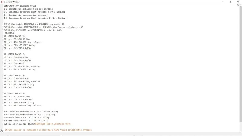
P1 = input ('ENTER the inlet PRESSURE at TURBINE (in bar): ' );
T1 = input ('ENTER the inlet TEMPERATURE at TURBINE (in Degree celsius): ');
P2 = input ('ENTER the PRESSURE at CONDENSER (in bar): ');
disp (' RESULTS');
%Getting the Cp & Cv values from Xsteam
%Cp & Cv are assumed not to changed with temperature to make numerical
%bit easy

%for vapour
CpV_high = XSteam('CpV_p', P1);
CpV_low = XSteam('CpV_p', P2);
CvV_high = XSteam('CvV_p', P1);
CvV_low = XSteam('CvV_p', P1);

%for liquid
CpL_high = XSteam('CpL_p', P1);
CpL_low = XSteam('CpL_p', P2);
CvL_high = XSteam('CvL_p', P1);
CvL_low = XSteam('CvL_p', P1);

%getting inportant parameters
%for high pressure
Tsat1 = XSteam('Tsat_p',P1);
Sg1 = XSteam('sV_p',P1);
Sf1 = XSteam('sL_p',P1);
Sfg1 = Sg1 - Sf1;
Hf1 = XSteam('hL_p',P1);
Hg1 = XSteam('hV_p',P1);
Hfg1 = Hg1 - Hf1;
%for low pressure
Sg2 = XSteam('sV_p',P2);
Sf2 = XSteam('sL_p',P2);
Sfg2 = Sg2 - Sf2;
Tsat2 = XSteam('Tsat_p',P2);
Hf2 = XSteam('hL_p',P2);
Hg2 = XSteam('hV_p',P2);
Hfg2 = Hg2 - Hf2;

%%%STATE Point 1

disp('AT STATE POINT 1:');

fprintf('P1 is : %f Bar \n', P1);

fprintf('T1 is : %f Deg celsius \n', T1);

H1 = XSteam('h_pt', P1, T1);
fprintf('H1 is : %f kJ/kg \n', H1);

S1 = XSteam('s_pt',P1, T1);
fprintf('S1 is : %f kJ/kg \n\n', S1);

%%%STATE Point 2

disp('AT STATE POINT 2:');

fprintf('P2 is : %f Bar \n', P2); % P2 input already taken

S2 = S1;
fprintf('S2 is : %f kJ/kg \n',S2);
%predicting location of point 2 in T-S
if (S2<= Sg2)
    X2 = (S2 - Sf2)/(Sfg2); %Dryness fraction at state point 2
else 
    X2 = 1;
end

fprintf ('X2 is : %f \n',X2);
%calculating T2 for superheat or weyt or dry wherevr itlies on the curve 
if (X2<1)
   T2 = Tsat2;
else
    %T2 calculated by S2 = Sg2+low_cpV*(log(T2/Tsat2))
    T2 = (Tsat2 + 273.15)*exp((S2-Sg2)/CpV_low); %"2 in superheated region"
    T2 = T2 - 273.15;
end
fprintf('T2 is : %f Deg celcius \n', T2);

if (X2 < 1)
    H2 = Hf2 + X2 * Hfg2;
else
    H2 = Hg2 + CpV_low*(T2-Tsat2);
end
fprintf('H2 is : %f kJ/kg \n\n', H2);

%%% STATE Point 3
%assuming no subcooling in condensor
disp('AT STATE POINT 3:');

P3 = P2;
fprintf('P3 is : %f Bar \n',P3);

V3 = XSteam('vL_p', P3);

T3 = Tsat2; % no subcooling assumed
fprintf('T3 is : %f Deg celsius \n',T3);

H3 = Hf2;
fprintf('H3 is : %f kJ/kg \n',H3);

S3 = Sf2;
fprintf('S3 is : %f kJ/kgk \n\n',S3);

%%%STATE Point 4
disp('AT STATE POINT 4:');

P4 = P1;
fprintf('P4 is : %f Bar \n',P4);

S4 = S3;
fprintf('S4 is : %f kJ/kgk \n',S4);

Wp = V3 * (P4 - P3) *100;
H4 = Wp + H3;
fprintf('H4 is : %f kJ/kg \n',H4);
% to calculate T4 S4 = S3 = Sf1 - CpL_high*ln(Tsat1/T4)
term = exp ((Sf1 - S4)/(CpL_high)); %use exp instead of Exp to take input as double 
T4 = Tsat1/term;
fprintf('T4 is : %f Deg celsius \n\n',T4);

%%workdone, heat,SSC and efficiency calculations 
Wt = H1 - H2;
fprintf('WORK DONE BY TURBINE is : %f kJ/kg \n', Wt);
fprintf('WORK DONE BY COMPRESSOR is %f kJ/kg \n', Wp);
Wnet = Wt - Wp;
fprintf('NET WORK DONE is : %f kJ/kg \n', Wnet);
Qin = H1 - H4;
n_thermal = (Wnet / Qin) * 100; %THERMAL EFFICIENCY
fprintf('THERMAL EFFICIENCY is : %f',n_thermal); disp(' % ');
SSC = 3600 / Wt ;  %SPECIFIC STEAM CONSUMPTION
fprintf('S.S.C. is %f kg/kwh', SSC);

%%calculations for plotting liqiud and vapour lines

%<>
%
TEMP = linspace(1, 373, 500);
for i = 1 : length(TEMP)
    H_L(i) = XSteam('hL_T', TEMP(i));
    H_V(i) = XSteam('hV_T', TEMP(i));
    S_L(i) = XSteam('sL_T', TEMP(i));
    S_V(i) = XSteam('sV_T', TEMP(i));
end
% Plotting T-S AND H-S Graphs
figure(1) %T-S
hold on
plot([S1 S2], [T1 T2],'r','linewidth',1)
text(S1,T1,' 1')
text(S2, T2, ' 2')
plot([S2 Sg2], [T2 Tsat2],'r','linewidth',1)
text (Sg2, Tsat2,' 2s')
plot([Sg2 S3], [Tsat2 T3],'r','linewidth',1)
text (S3, T3,' 3')
plot([S3 S4], [T3 T4],'r','linewidth',1)
text (S4, T4,' 4')
plot([S4 Sf1],[T4 Tsat1],'r','linewidth',1)
text (Sf1, Tsat1',' 4s')
plot([Sf1 Sg1], [Tsat1 Tsat1],'r','linewidth',1)
text (Sg1, Tsat1,' 1s')
plot([Sg1 S1], [Tsat1 T1],'r','linewidth',1)
plot(S_L,TEMP, '--b')
plot(S_V,TEMP, '--b')
%%Marking Directions
text(S1, (T1 + T2)/2, 'v','HorizontalAlignment','center','color','black')
text((Sg2+Sf2)/2,  T3, '<', 'color', 'black')
text(S3,(T3+T4)/2, '^','HorizontalAlignment','center','color','black','linewidth',1.5)
text((Sf1+Sg1)/2, Tsat1, '>','color','black')
title ('T-S DIAGRAM OF IDEAL RANKINE CYCLE','fontsize',15)
ylabel('TEMPERATURE (DegC)')
xlabel('SEPCIFIC ENTROPY (kJ/kgk)')
axis([0 15 0 450]);
%H-S
figure(2) 
hold on
plot([S1 S2], [H1 H2],'r','linewidth',1)
text(S1,H1,' 1')
plot([S2 S3], [H2 H3],'r','linewidth',1)
text(S2,H2,' 2')
plot([S3 S4], [H3 H4],'r','linewidth',1)
text(S3,H3,' 3')
plot([S4 S1], [H4 H1],'r','linewidth',1)
text(S4,H4,' 4')
plot(S_L, H_L,'b--','linewidth',1)
plot(S_V, H_V,'b--','linewidth',1)
title('H-S DIAGRAM','fontsize',15)
ylabel('SPECIFIC ENTHALPY (kJ/kg)')
xlabel('SPECIFIC ENTROPY (kJ/kgk)')