Week 3 - Solving second order ODEs

Aim- Writing the programme to solve the following ODE,

D2theta/dt2 + (b/m)*dtheta/dt-(g/l)*sin(theta) = 0

This ode represents the equation of motion of simple pendulum with damping.

Objective – To know how pendulum oscillates, & on which factors it depends. By solving given second order ODE.

Equations- D2theta/dt2 + (b/m)*dtheta/dt-(g/l)*sin(theta) = 0

Program codes explanation –

1. clear all – It is used to clear all the variables inserted from the work space.
2. Close all – It is used to clear or close opened figures or images.
3. Clc – It is used to command window.

Inputs provided –

b = damping factor

g = gravitational force

l = length of pendulum

= mass of pendulum

Damping – It is an internal force of an oscillatory system which acts against the oscillations of the system and tries to reduce or prevent the systemn from oscillations.

Damping ratio - It is the parameter which characterize the frequency response of a second order ordinary differential equation.

Pendulum – It is a weight suspended from a pivot so that it can swing freely when released, the restoring force acting on the pendulum mass causes it to oscillate about the equilibrium position swinging back & forth.

The time for one complete cycle of a left swint & right swing is called the period.

Length of pendulum – Length of pendulum is directly proportional to the period of oscillation.

Mass of pendulum – The mass of pendulum does not affect the oscillation of pendulum because the mass and the force (acceleration due to gravity) are directly proportional to each other.

Initial conditions – (theta_0) = (0, 3)

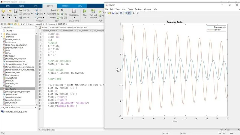
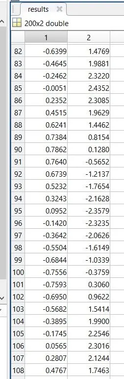
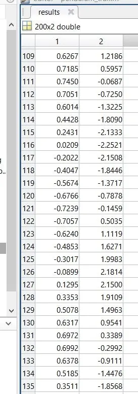
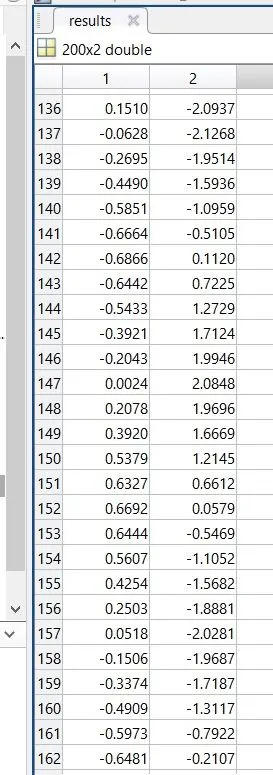
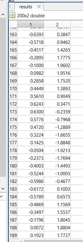
These are the conditions provided in which 0 is the initial displacement and velocity is 3 meter per sec.

Time span - (t_span) =linspace (0, 20, 200)

It will give us the time span as per which the velocity changes (linspace(starting time, ending time, 200 values)

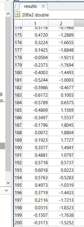
[t, results] = ode45(@(t, theta) ode_func(t, theta, b, g, l, m), t_span, theta_0)

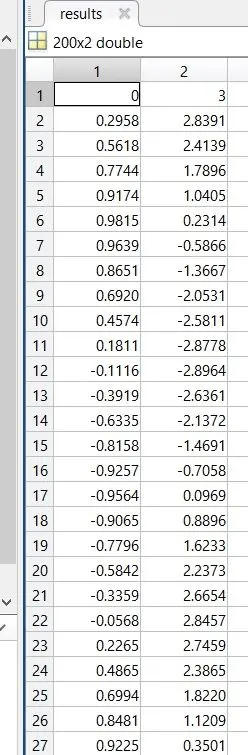
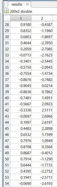
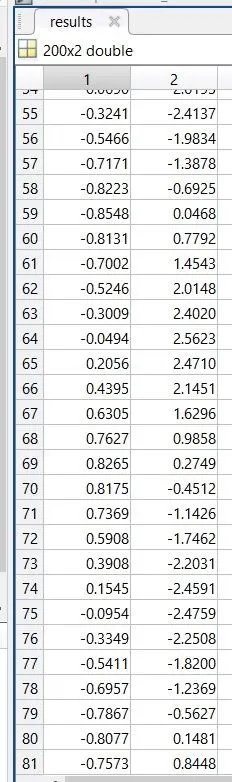
[t, results] = Result vector which will gives the column vector containing 2 column one is displacement and one is velocity.

Ode45 = it is the inbuild solver of matlab for derivative

(t, theta) = these are the inputs on which ode depends

Ode_func = It is the function we are using to give the inputs and defining them

(t, theta, b, l, m,) these are the inputs

T = Time

Theta = Angle changed with respect to time (angle between pendulum rod and the normal drawn from pivote of pendulum.

B = damping factor

L = length of pendulum

M = mass of pendulum.

Function [dtheta_dt] it the array of 2 first order derivatives

Dtheta_dt = theta2

Dthet2_dt = -(b/m)*theta2-(g/l)*sin(theta1)

Ct=1 (counter)(which represent each and every frame we creating)

For_loop – It will use the explained values one after one. For i = 1 : length(t_span)

In this for loop is for from 1 to the length of t_span i.e. for the time span of 1 to 20 sec. with 200 values in between.

Here we are using ‘for_loop’ to get the different positions of the pendulum which depends on the theta and displacement and displacement depends on time.

After writing for loop for link we have to insert the calculation part for positioning the links.

Plotting – In this we make a counter (ct=1) and after ‘for_loop’ we’ll incrementing that by ct=ct+1.

Plot ([x0 x1], [y0 y1], ‘linewidth’,2, ‘color’, ‘b’)

In this,

plot ([x coordinate of first link], [y coordinates of first link],’width of line command’, line width in mm, ‘color of line’, ‘blue’)

plot(x1,y1, ‘marker’, ‘o’. ‘markersize’,15, ‘markerfacecolor’, ‘r’)

In this,

The marker command is used t represent the pendulum ball of ‘o’ shape,size of 15 mm and color of red

Also I have given some points for plotting those points represent the support wall where the pendulum is pivoted.

Axis command is used to fix our axis limits. (start and end points of our axis.

Axis(-3.0 3 0 3)

Means our x-axis will display coordinates from -2 to 2 and y-axis will display from -1.5 to 1.

For creating movie we have to create an array containing our frames (ct)

mp(ct) = getframe(gcf) (NOTE- getframe command is must be used before incrementation of counters which will save previous frame and then that’s get incremented by one.)

getframe command will gather all the frames (getting current figure window)

for creating a movie we will use the command

movie(mp) = movie(name)

videofile = videowriter(name of file and profile)

open(videofile)

write(videofile,m)

close(videofile)

“for making movie we have to create a video file using command video writer ( contains name of file with format of file, and profile compressed or uncompressed)

Open – it will open the video file

Write – we will be writing the frames we captured in array ‘m’

And close command will close the video file.

The video will be saved in the program folder which we can play using any media player.

Mathematical Explanations – ODE are very important part of any system after solving ode we can understand the system phenomena.

In this given ODE we can understand that oscillation of the pendulum is dependent of velocity and the displacement and the velocity changes w.r.t. time.

The given ODE is 2^nd order ODE hence we have to break this into set of first order ODE.

Given equation,

(d2 theta/ dt2) +(b/m)*(dtheta/dt)+(g/l)*sintheta = 0

For breaking this,

Consider,

theta = theta1

dtheta/dt = dtheta1/dt = theta2 -------------I

d2theta/dt2 = d2theta1/dt2 = d/dt(dtheta1/dt) = d/dt(theta2) -----------II

substituting the values we get,

dtheta1/dt = theta2 ------- first order equation

dtheta2/dt = -(b/m)theta2 – (g/l)sintheta1 --------- first order equation.

Conclusion – Hence we solved the given second order equation and understand the mathematics behind the pendulum. Oscillation of the pendulum depends on the damping factor as well as length of pendulum.

clear all
close all
clc

%pendulum animation 
%inputs l=length of string (meter)
% b=damping coefficient
% g=gravitational force
% m=mass of ball
%inputs 
b = 0.05;
g = 9.81;
l = 1;
m = 1;

%initial condition theta_0 = [angular displacement, velocity]
theta_0 = [0, 3];

%time points
t_span = linspace (0,20,200);

%solve ODE

[t, results] = ode45(@(t,theta) ode_func(t, theta, b,g,l,m), t_span, theta_0);
% plot (t, results(:, 1))
% hold on
% plot (t, results(:, 2))
% ylabel ('plot')
% xlabel ('time')
% legend('Displacement','velocity')
% title('Damping factor')
ct = 1;
for i = 1:length(t_span);
    x0 = 0;
    y0 = 0;
    x1 = l*sin(results(i, 1));
    y1 = -l*cos(results(i, 1));
    %following plot is the rod of pendulum
    plot([x0, x1],[y0, y1], 'linewidth',2,'color','b')
    hold on
    %following polt is for support for pivote
    plot ([-1, 1],[0, 0],[-1, -0.75],[0,0.25],[-0.75, -0.5],[0,0.25],[-0.5, -0.25],[0,0.25],[-0.25, 0],[0,0.25],[0, 0.25],[0,0.25],[0.25, 0.5],[0,0.25],[0.5, 0.75],[0,0.25],[0.75, 1],[0,0.25],[1, 1.25],[0,0.25], 'linewidth',2,'color','black')
    %following plot is for pendulum ball 
    plot(x1,y1,'marker', 'o','markersize',15,'markerfacecolor','r');
    hold off
    axis ([-2 2 -1.5 1])
    MP(ct) = getframe(gcf);
    ct = ct+1;
end

movie(MP)
videofile=VideoWriter('pendulum.avi','uncompressed avi');
open(videofile)
writeVideo(videofile,MP)
close(videofile)

function [dtheta_dt] = ode_func(t, theta, b,g,l,m)

theta1 = theta(1)
theta2 = theta(2)
dtheta1_dt = theta2;
dtheta2_dt = -(b/m)*theta2-(g/l)* sin(theta1);
dtheta_dt = [dtheta1_dt ; dtheta2_dt];
end