Week 4.1 - Genetic Algorithm

Aim: To write a code in MATLAB to optimise the stalagmite function and find the global maxima of the function.

Theory:

Genetic Algorithm:

A genetic algorithm is a method of solving both constrained and unconstrained optimization problems based on a natural selection process that mimics biological evolution. The algorithm repeatedly modifies a population of individual solutions. At each step, the genetic algorithm randomly seletcs individuals from the current population and uses them as parents to produce the children for next generation. Over successive generations, the population evolves towards an optimal solution. You can apply the genetic algorithm to solve problems that are not well suited for standard optimization algorithms, including problems in which the objective function is discontinuous, nondifferentiable, stochastic, or highly nonlinear.

Mentioned below are five main phases of Genetic Algorithm:

• Initialization of Population
• Fitness Function
• Selection
• Crossover
• Mutation

Working of Genetic Algorithm:

1. The algorithm begins by creating a random initial population.
2. The algorithm then creates a sequence of new populations. At each step, the algorithm uses the individuals in the current generation to create the next population.
3. The algorithm stops when one of the stopping criteria is met.
4. The algorithm takes modified steps for linear and integer constraints.
5. The algotithm is further modified for nonlinear constraints.

Stopping Criteria:

The genetic algorithm uses the following options to determine when to stop.

1. MaxGenerations - The algorithm stops when the number of generations reaches MaxGenerations.
2. MaxTime - The algorithm stops after running for an amount of time in seconds equal to MaxTime.
3. FitnessLimit - The algorithm stops when the value of the fitness function for the best points in the current population is less that or equal to FitnessLimit.
4. MaxStallGenerations - The algorithm stops when the average relative change in the fitness function value over MaxStallGenerations is less than Function tolerance.
5. MaxStallTime - The algorithm stopes if there is no improvement in the objective function during an interval of time in seconds equal to MaxStallTime.
6. FunctionTolerance - The algorithm runs until the average relative change in the fitness function value over MaxStallGenerations is less than Function tolerance.
7. ConstraintTolerance - The ConstraintTolerance is not used as stopping criteria. It is used to determine the feasibility with respect to nonlinear constraints.

Genetic Algorithm Syntax:

x = ga(fun,nvars)

x = ga(fun,nvars,A,b)

x = ga(fun,nvars,A,b,Aeq,beq)

x = ga(fun,nvars,A,b,Aeq,beq,lb,ub)

x = ga(fun,nvars,A,b,Aeq,beq,lb,ub,nonlcon)

x = ga(fun,nvars,A,b,Aeq,beq,lb,ub,nonlcon,options)

x = ga(fun,nvars,A,b,Aeq,beq,lb,ub,nonlcon,intcon)

x = ga(fun,nvars,A,b,Aeq,beq,lb,ub,nonlcon,intcon,option)

x = ga(problem)

[x,fval] = ga(_)

[x,fval,exitflag,output] = ga(_)

[x,fval,exitflag,output,population,scores] = ga(_)

The Main code for all three studies:

clear all
close all
clc

x=linspace(0,0.6,150);
y=linspace(0,0.6,150);
n_cases=50;

[xx,yy]=meshgrid(x,y);

for i=1:length(xx)
    for j=1:length(yy)
        input_vector(1)=xx(i,j);
        input_vector(2)=yy(i,j);
        stal(i,j)=stalagmite(input_vector);
    end
end

surfc(xx,yy,stal)
xlabel('x value');
ylabel('y value');

shading interp

[inputs,fval] = ga(@stalagmite,2);

tic
%%Study 1 (Behaviour without boundary conditions)
for k=1:n_cases
    [inputs,fopt(k)]=ga(@stalagmite,2);
    xopt(k)=inputs(1);
    yopt(k)=inputs(2);
end
study_time=toc;

figure(1)
subplot(2,1,1)
hold on
surfc(x,y,-stal)
shading interp
plot3(xopt,yopt,-fopt,'marker','o','MarkerSize',5,'MarkerFaceColor','r')
title('Unbounded inputs')
subplot(2,1,2)
plot(-fopt)
xlabel('Iterations')
ylabel('Function minimum')

tic
%%Study2 (with upper and lower bounds)

for k=1:n_cases
    [inputs,fopt(k)]=ga(@stalagmite,2,[],[],[],[],[0;0],[0.5;0.5]);
    xopt(k)=inputs(1);
    yopt(k)=inputs(2);
end 
study_time_2=toc;

figure(2)
subplot(2,1,1)
hold on
surfc(x,y,-stal)
shading interp
plot3(xopt,yopt,-fopt,'marker','o','MarkerSize',5,'MarkerFaceColor','r')
title('Bounded Inputs')
subplot(2,1,2)
plot(-fopt)
xlabel('Iterations')
ylabel('Function minimum')

%Study 3 (Increasing the GA Iterations)
options=optimoptions('ga');
options=optimoptions(options,'PopulationSize',170);

tic
for k=1:n_cases
    [inputs,fopt(k)]=ga(@stalagmite,2,[],[],[],[],[0,0],[0.5,0.5],[],[],options);
    xopt(k)=inputs(1);
    yopt(k)=inputs(2);
end

study_time_3=toc;
figure(3)
subplot(2,1,1)
hold on
surfc(x,y,-stal)
shading interp
plot3(xopt,yopt,-fopt,'marker','o','markersize',5,'markerfacecolor','r')
title('Increased Iterations')
subplot(2,1,2)
plot(-fopt)
xlabel('Iterations')
ylabel('function minimum')

Stalagmite Function:

The formula mentioned below is used in this function.

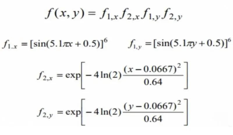
The Stalagmite Fuction code used in this program:

function stal = stalagmite(input_vector)

x=input_vector(1);
y=input_vector(2);

fonex=(sin(5.1*pi.*x+0.5)).^6;
foney=(sin(5.1*pi.*y+0.5)).^6;

ftwox=exp(-4*log(2).*(((x-0.0667).^2)./0.64));
ftwoy=exp(-4*log(2).*(((y-0.667).^2)./0.64));

stal = -((fonex)*(foney)*(ftwox)*(ftwoy));
end

Figure 1 -

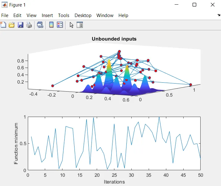
Figure 2 -

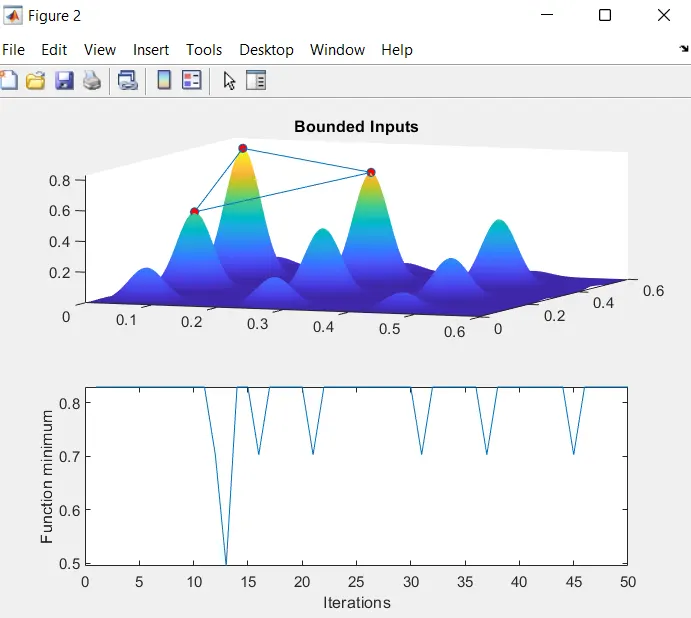
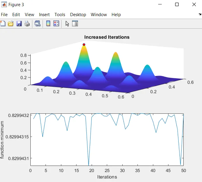
Figure 3 -

Step-wise explanation of the code used in this program:

1. Firstly, The code starts of with the command 'clear all' to clear the data stored in the workspace, 'close all' to close all the plots and figures, and 'clc' to clear the command window.
2. Then the 'x' and 'y' array is defined using the 'linspace' command to create values at 150 equal intervals.
3. The 'meshgrid' command is used for creating a 2D mesh of x and y array.
4. The number of iterations the code should performed is then defined as 50. (i.e, n = 50)
5. The input vector values 'xx' and 'yy' are defined and even the stalagmite function for these input vectors.
6. In the next step 3 study cases need to be performed in which, the first study case is carried out with no boundary conditions.
7. The 'for' loop command is used using the 'ga' syntax to give values for inputs and optimum max value. The 'stalagmite' function is called in along with the number of variables.
8. And to know the time taken to solve these iterations the 'tic and tok' command is used.
9. Further to plot the function the 'surfc' command is used. And for multiple plots the 'subplot' command is used.
10. The 'shading interp' command is used to remove the gridlines from the surface and to obtain a smooth and clear plot.
11. Then the 'plot3' command is used to plot the 3D points at 'xopt','yopt' and '-fopt' with a 'o' shaped marker with a defined markersize 5 and marker face color as red.
12. Study case 2 is further carried out to avoid obtaining different results every time the program was carried out by simply specifying the upper and lower bounds. It's done by adding the upper limits "[0;0]" and lower limits "[0.5;0.5]" to the 'ga' syntax mentioned in above.
13. Then again using the 'plot3' command we can plot the 2nd study case and it is observed that the results are not same every time we run the program.
14. The solution to solve this program is to increase the number aof iterations. Therefore In study case 3 the number of iterations was increased to 170 by using the 'option' syntax. In study 3 the 'ga' syntax is similar to study 1 and 2 but difference is that it contains 'option' term.

References:

https://in.mathworks.com/help/gads/what-is-the-genetic-algorithm.html

https://in.mathworks.com/discovery/genetic-algorithm.html

How the Genetic Algorithm Works - MATLAB & Simulink - MathWorks India