Week 4.1 - Genetic Algorithm
Genetic Algorithm:
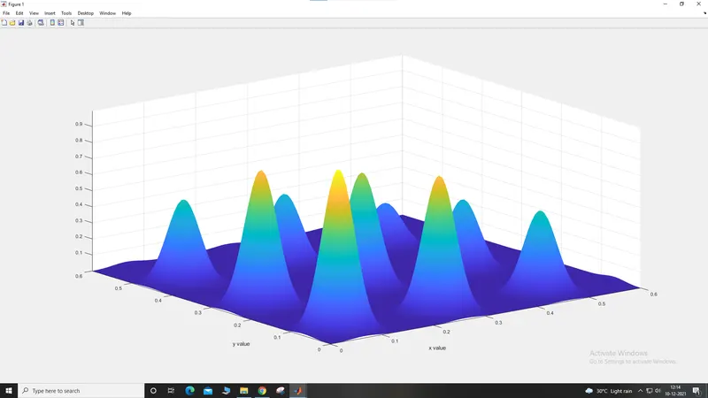
Aim: To write a code in MATLAB to optimize the stalagmite function and to find the global maxima of the function.
Given:
`f1,x=[sin(5.1pix+0.5)]^6`
`f1,y=[sin(5.1piy+0.5)]^6`
`f2,x=exp[-4ln(2)(x-0.0667)^2/0.64]`
`f2,y=exp[-4ln(2)(y-0.0667)^2/0.064]`
`f(x,y)=f1,x*f2,x*f1,y*f2,y`
To use this formula to code a stalagmite function.
GA syntax:
x = ga(fun,nvars)
x = ga(fun,nvars,A,b)
x = ga(fun,nvars,A,b,Aeq,beq)
x = ga(fun,nvars,A,b,Aeq,beq,lb,ub)
x = ga(fun,nvars,A,b,Aeq,beq,lb,ub,nonlcon)
x = ga(fun,nvars,A,b,Aeq,beq,lb,ub,nonlcon,options)
x = ga(fun,nvars,A,b,Aeq,beq,lb,ub,nonlcon,intcon)
x = ga(fun,nvars,A,b,Aeq,beq,lb,ub,nonlcon,intcon,options)
x = ga(problem)
[x,fval] = ga(___)
[x,fval,exitflag,output] = ga(___)
[x,fval,exitflag,output,population,scores] = ga(___)
Syntax explnation:
x = ga(fun,nvars)
- fun = function handle or function names
- nvars = Number of variables specified as positive integers
x = ga(fun,nvars,A,b)
- A = Linear inequality constraints, specified as real matrix
- B = linear inequality constraints, specified as real vector
x = ga(fun,nvars,A,b,Aeq,beq)
x = ga(fun,nvars,A,b,Aeq,beq,lb,ub)
- lb = Lower bounds, spacified as real vector or array
- ub = upper bounds
x = ga(fun,nvars,A,b,Aeq,beq,lb,ub,nonlcon)
- nonlcon = Non linear constraints, specified as function handle or function name. It is a function that accepts a vector or array x and returns two arrays c(x) and ceq(x)
x = ga(fun,nvars,A,b,Aeq,beq,lb,ub,nonlcon,options)
- options = optimization options, specified as output optimization or a structure
x = ga(fun,nvars,A,b,Aeq,beq,lb,ub,nonlcon,intcon)
- intcon = integer variables
x = ga(fun,nvars,A,b,Aeq,beq,lb,ub,nonlcon,intcon,options)
x = ga(problem)
- ga(problem) = problem description specified as structure
[x,fval] = ga(___)
- Returns the value of fitness function x
[x,fval,exitflag,output] = ga(___)
- exitflag = When there are integer constraints, ga uses the penalty fitness value instead of the fitness value for stopping criteria
[x,fval,exitflag,output,population,scores] = ga(___)
- population= Final population returned as a PopulationSize
- scores = For non integer problems the final scores are the fitness function values of row population and for integer problems the final scores are the penalty fitness values of the population members
Program code:
clear all
close all
clc
num_cases = 50

%defining search space
x = linspace (0, 0.6, 150);
y = linspace (0, 0.6, 150);

%creating 2D mesh
[xx yy] = meshgrid(x, y);

%Evaluating the stalagmite function
for i = 1:length(xx)
    for j = 1:length(yy)
        input_vector(1) = xx(i, j);
        input_vector(2) = yy(i, j);
        f(i, j) = stalagmite(input_vector);
    end
end

surfc(xx, yy, -f)
xlabel('x value')
ylabel('y value')
shading interp;


tic
%Study 1 - Statistical behavior
for i = 1:num_cases
    [inputs, fopt(i)] = ga(@stalagmite, 2);
    xopt(i) = inputs(1);
    yopt(i) = inputs(2);
end
study1_time = toc
figure(2)
subplot(2,1,1)
hold on
surfc(x, y, -f)
shading interp
plot3(xopt, yopt, -fopt, 'marker', 'o', 'markersize', 5, 'markerfacecolor', 'r')
title('Unbounded inputs')
subplot(2,1,2)
plot(-fopt)
xlabel('Iterations')
ylabel('Function minimum')

tic
%Study 2 - Statistical behavior with upper bounds and lower bounds
for i = 1:num_cases
    [inputs, fopt(i)] = ga(@stalagmite, 2, [], [], [], [],[0;0], [0.6;0.6]);
    xopt(i) = inputs(1);
    yopt(i) = inputs(2);
end
study2_time = toc
figure(3)
subplot(2,1,1)
hold on
surfc(x, y, -f)
shading interp
plot3(xopt, yopt, -fopt, 'marker', 'o', 'markersize', 5, 'markerfacecolor', 'r')
title('Bounded Inputs')
subplot(2,1,2)
plot(-fopt)
xlabel('Iterations')
ylabel('Function minimum')


%Study 3 - Increasing GA iterations
options = optimoptions('ga')
options = optimoptions(options, 'PopulationSize', 300);
tic
for i = 1:num_cases
    [inputs, fopt(i)] = ga(@stalagmite, 2, [], [], [], [], [0;0], [0.6;0.6], [],[], options);
    xopt(i) = inputs(1);
    yopt(i) = inputs(2);
end
studty3_time = toc
figure(4)
subplot(2,1,1)
hold on
surfc(x,y,-f)
shading interp
plot3(xopt, yopt, -fopt, 'marker', 'o', 'markersize', 5, 'markerfacecolor', 'r')
title('Bounded inputs with increased population size')
subplot(2,1,2)
plot(-fopt)
xlabel('Iterations')
ylabel('Function minimum')
Function program:
function f = stalagmite(input_vector)
x = input_vector(1);
y = input_vector(2);
f1 = (sin(5.1*pi*x+0.5))^6;
f2 = (sin(5.1*pi*y+0.5))^6;
f3 = exp(-4*log(2)*(x-0.0667)^2/0.64);
f4 = exp(-4*log(2)*(y-0.0667)^2/0.64);
f = -(f1*f2*f3*f4);
end
Output:
GA output:
Study 1:
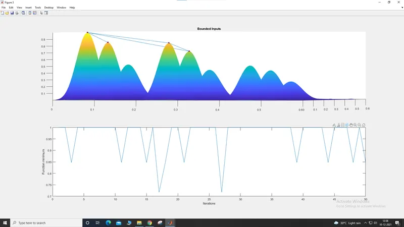
Study 2:
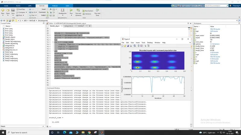
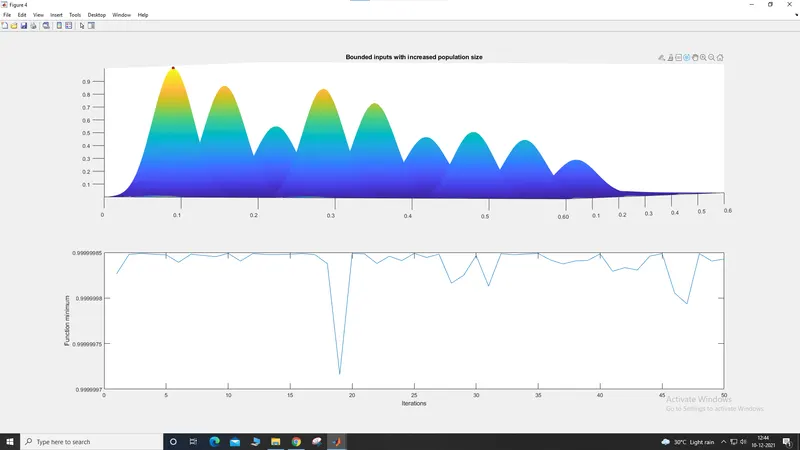
Study 3:
Explanation:
- Line 6 - 8: Input arrays x = linspace(0,0.6,150) and y = linspace(0, 0.6, 150) ga does not define search space.
- Line 10 - 11: 2D mesh is created using meshgrid command.
- Line 13 - 20: Evaluating the stalagmite function using for loops.
- Line 22: Surfc command is used to create 3D surface plot.
- Line 23 - 24: Labeling commands are used.
- Line 25: shading interp function is used to color shade the surface, it varies the color in each line segment.
- Line 28 and 35 Tic and toc commands is used to determine the evaluation time.
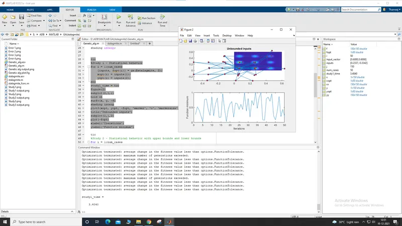
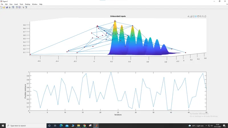
- Line 29 - 34: for loop for study 1 is created.
- Line 37: Subplot function is used for having multiple plots inside same figure window.
- Line 41: plot3 function is used to plot 3D coordinateds in space.
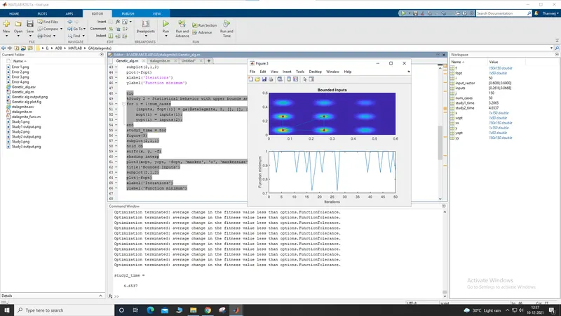
- Line 48 - 66: Study 2 is created and evaluated using upper bound and lower bounds, due to small initial population value MATLAB found the local maxima instead of global maxima.
- Line 70: Options functions is used optimize ga
- Line 71 - 77: Polulation size is increased and for loop is created and bounds are specified.
Function program is slightly modified to get the values greater than 0. To get maximum value of stalagmite function (-ve) is has been used, hence ga finds global maxima if not the plot looks inverted and it will find global minima.
Errors:
Error 1:
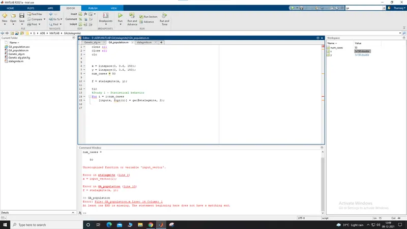
Input vector was not recognized because it wan not defined in the program. Hence it was rectified.
Error 2:
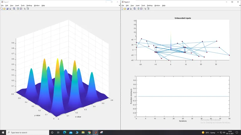
The plot was marked at 0 when evaluated and it was rectified.
Error 3:
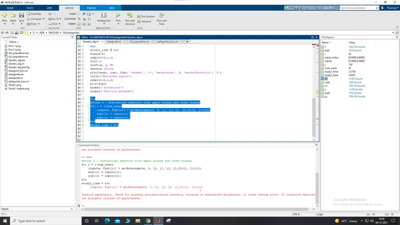
Upper bound limit was wrongly entered and it was rectified.
Error 4:
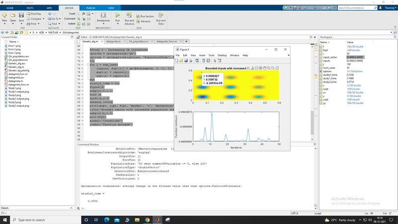
when evaluated the study the time in the comand window was 0.3 sec which was wrong because when the population size was increased MATLAB take time to evaluate it, when analyzed for loop was not specified with 1:num_cases, then it was rectified.
Conclusion:
Hence global maxima was found by creating stalagmite function using ga in MATLAB.
Reffrence: