Week 3 - Solving second order ODEs

Aim: To solve the program that solves ODE and create an output for simple pendulum.

Given data: `d^2/dt + b/m d theta/dt + g/L sin theta=0`

here,

g = gravity in m/s2

L = length of the pendulum in m

m = mass of the ball in kg

b=damping coefficient

To use,

L=1 metre

m=1 kg

b=0.05

g=9.81 m/s2

angular velocity = 3rad/sec

Program code:

MAIN PROGRAM

clear all 
close all
clc

b = 0.05;
g = 9.81;
l = 1;
m = 0.1;

%initial condition
theta_0 = [0;3];

%time points
t_span = linspace (0,15,500);
ct = 1;

%solve ODE
[t,results] = ode45(@(t,theta) ode_func(t,theta,b,g,l,m),t_span,theta_0);
 
%plotting
 figure(1)
 plot(t,results(:,1))
 hold on
 plot(t,results(:,2))
 ylabel('plot')
 xlabel('time')
 grid on 
 ct = 1;
 hold off
    
 %pendulum
 figure(2)
 for i = 1:length(t_span)
     x0 = 0;
     y0 = 0;
     x1 = 1*sin(results(i,1));
     y1 = -l*cos(results(i,1));
     plot([x0 x1], [y0 y1], 'linewidth', 3)
     hold on
     plot ([-1.5 1.5], [0 0], 'linewidth', 3)
     
     %plotting pendulum bob
     plot(x1,y1,'o','markersize',10,'markerfacecolor','b')
     
     %joining end points of line and fixed end
     plot(x0,y0,'o','markersize',6,'markerfacecolor','k');
     
     %connecting bob and fixed end
     plot([x0 x1], [y0 y1],'linewidth',2)
     axis ([-1.5 1.5 -1.5 1.5])
     
     M(ct) = getframe(gcf);
     ct = ct+1;
     hold off
 end
 
    
movie(M)
videofile = VideoWriter('ODE.avi','Uncompressed AVI');
open(videofile)
writeVideo(videofile, M)
close(videofile)

FUNCTION PROGRAM

function [dtheta_dt] = ode_func(t,theta,b,g,l,m)
theta1 = theta(1)
theta2 = theta(2)
dtheta1_dt = theta2;
dtheta2_dt = -(b/m)*theta2 - (g/l)*sin(theta1);
dtheta_dt = [dtheta1_dt;dtheta2_dt];
end

Step wise explanation of program code:

Line 1 - 3: Clear all, close all and clc commands are used.

Line 5: b = 0.05 where, "b" is the damping coefficient.

Line 6: g = 9.81 where, "g" is the gravity in `m/s^2`.

Line 7: l = 1 where, "l" is the length of the pendulum in `m`.

Line 8: m = 0.1 where, "m" is the mass bob in `kg`.

Line 10: Initial condition is applied with the unit of rad/sec.

Line 13 - 15: The condition for t_span is applied using linspace command and ct is entered.

Line 17: ODE is solved by calling in the function program, ODE45 is an inbuilt solver in MATLAB.

Line 20 - 29: The plots for figure(1) is entered and to bring the values from reults the column and row iteration is used. ylable and xlable is named as 'plot' and 'time'.

Line 31 - 40: The plot for figure(2) pendulum is entered, for loop is used. The value for i, x0, y0, x1, y1 is assigned and plot command and linewidth command is used.

Line 42 - 43: The pendulum bob is plotted and markersize and markerfacecolor command is used to determine the marker sized and color.

Line 45 - 46: The end points of line and fixed line are plotted and same markersize and markerfacecolor command is used.

Line 48 - 50: The plot for axis is created to connect bob and the fixed end.

Line 52 - 55: Getframe command is used and forloop is ended.

Line 58 - 62: commands to create animation file is entered.

Screenshots of errors faced while programming:

Error 1:

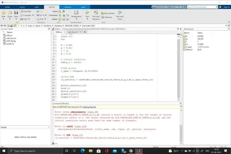
The initial condition vector must have the same number of elements.

Error 2:

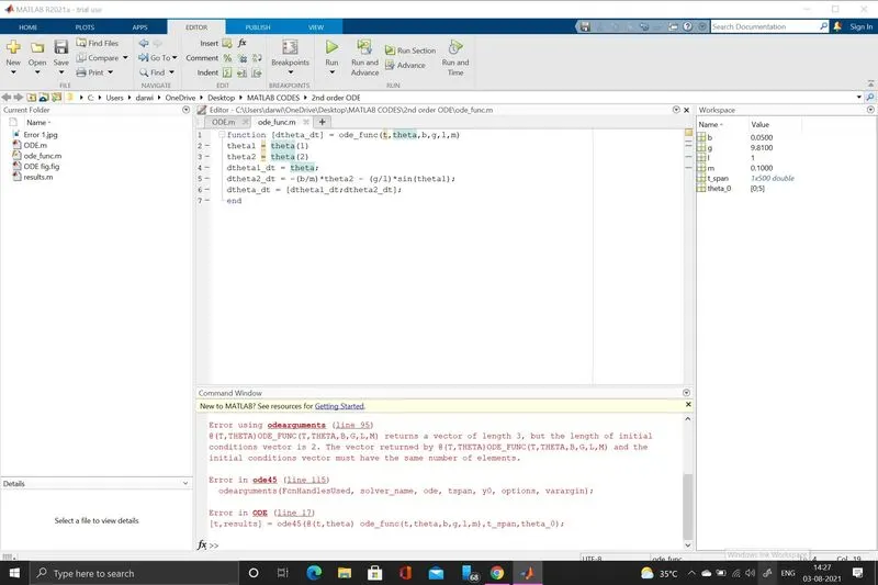
There was an error in function program and it was identifyed and corrected.

Error 3:

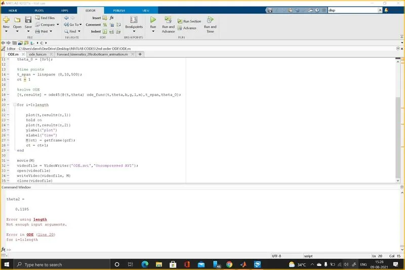There was not enough input arguments for length and it was corrected.

Error 4:

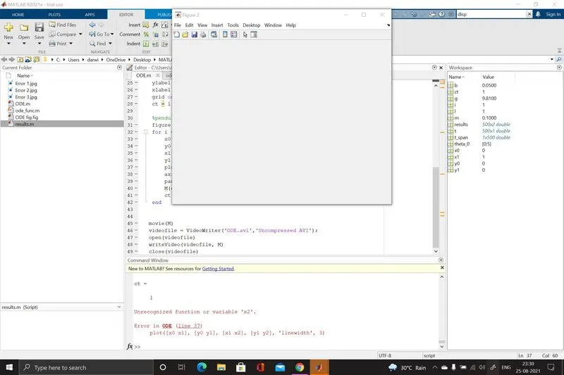
Unrecognized variable 'x2'. It was reviewd and corrected.

Error 5:

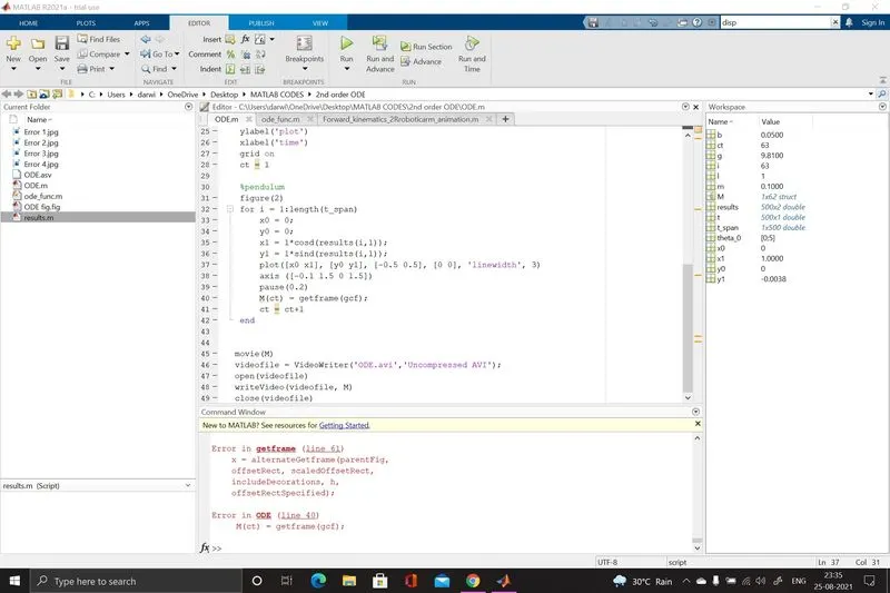
There was a error in getframe and it was corrected.

Error 6:

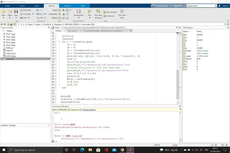
There was anerror while plotting. Markercolor was changed to markerfacecolor.

Error 7:

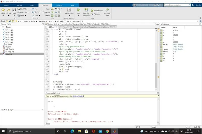
Invalid color or line style. Instead of '0' it was changed to 'o'.

Error 8:

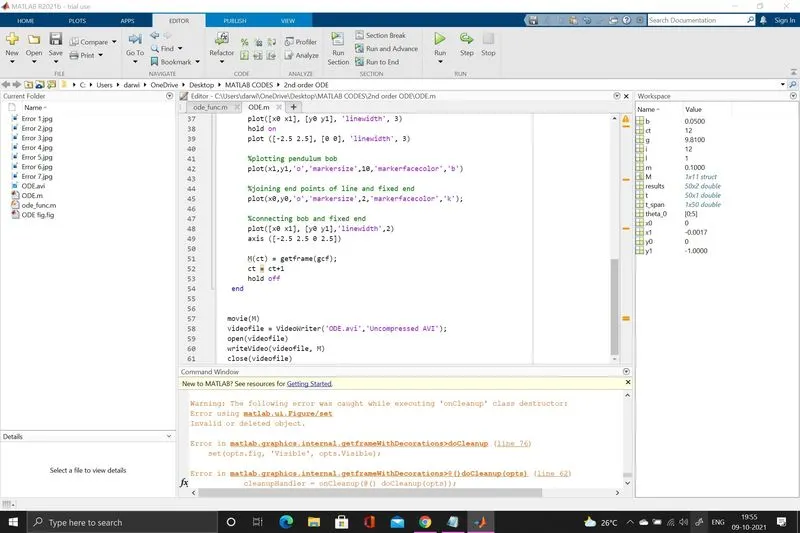
Invalid deleted object. The issue was solved.

Error 9:

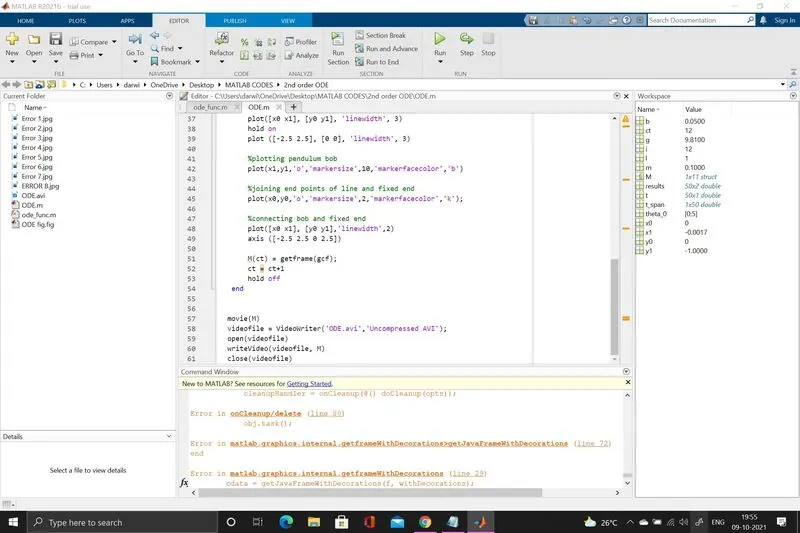
By mistake the running process was stopped so this error popped up and it was resolved.

Error 10:

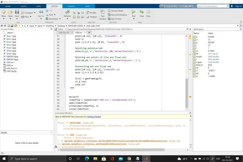
There was am error while playing the output and it was resolved.

Error 11:

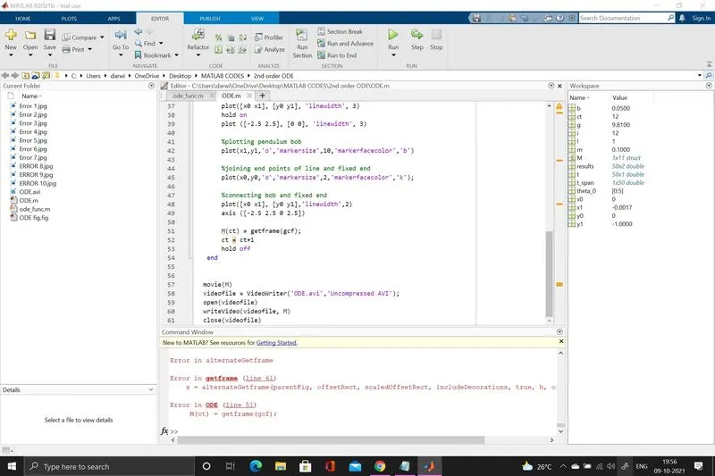
An alternate figure error appeared and it was corrected.

OUTPUT:

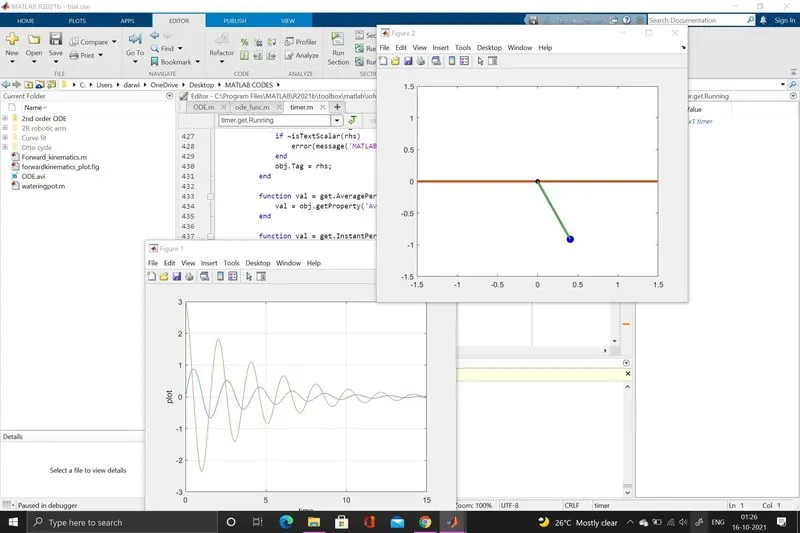
The plot couldn't be uploaded here so I've uploaded down.

Conclusion:

Hence the coed for simulating simple pendulum using ODE in MATLAB is created and output is displayed.