Week 4.1 - Genetic Algorithm

Aim: -

To calculate the global maxima of stalagmite function.

Introduction: -

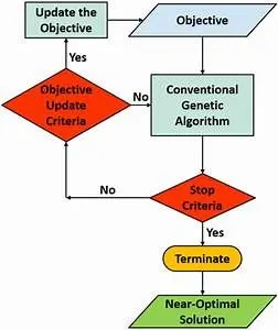
A Genetic algorithm is a search heuristic that mimics the process of natural evolution. This heuristic is routinely used to generate useful solutions to optimization and search problems. Genetic algorithms belong to the larger class of evolutionary algorithms, which generate solutions to optimization problems using techniques inspired by natural evolution, such as inheritance, mutation, selection, and crossover. Genetic algorithms find application in bioinformatics, phylogenetics, computational science, engineering, economics, chemistry, manufacturing, mathematics, physics, pharmacometrics and other fields.

The algorthim reflects the process of natural selection where the fittest individuals are selected for reproduction in order to produce offspring of the next generation.

Genetic Algorthim are primarily used in optimization problems of various kinds, but they are frequently used in other

application areas as well.

Stalagmite function used in the program is: -

f(x,y) = f1x. f2x. f1y. f2y

f1x = (sin(5.1*pi*x +0.5))^6

f1y = (sin(5.1*pi*y +0.5))^6

f2x = exp(-4ln2((x-0.0667)^2/0.64))

f2y = exp(-4ln2(y-0.0667)^2/0.64)

Three Cases perform in this project

(i) Study of Genetic Algorthim for the random sampling.

(ii)Study of Genetic Algorthim with upper and lower bound Sampling.

(iii)Study of Genetic Algorthim with upper and lower bound and increase the population size.

Case1:-Genetic Algorthim for the random sampling.

%Defining our search space
x = linspace(0,0.6,150);
y = linspace(0,0.6,150);

%creating a 2Dimensional mesh
[xx yy] = meshgrid(x,y);
n=150;

%Evaluating the stalagmite function
for i = 1:length(xx)
for j = 1:length(yy)
input_vector(1)=xx(i,j);
input_vector(2)=yy(i,j);
F(i,j)=stalagmite(input_vector);
end
end

tic
for i = 1:n
[inputs, Fopt(i)] = ga(@stalagmite,2);


xopt(i) = inputs(1);
yopt(i) = inputs(2);

end

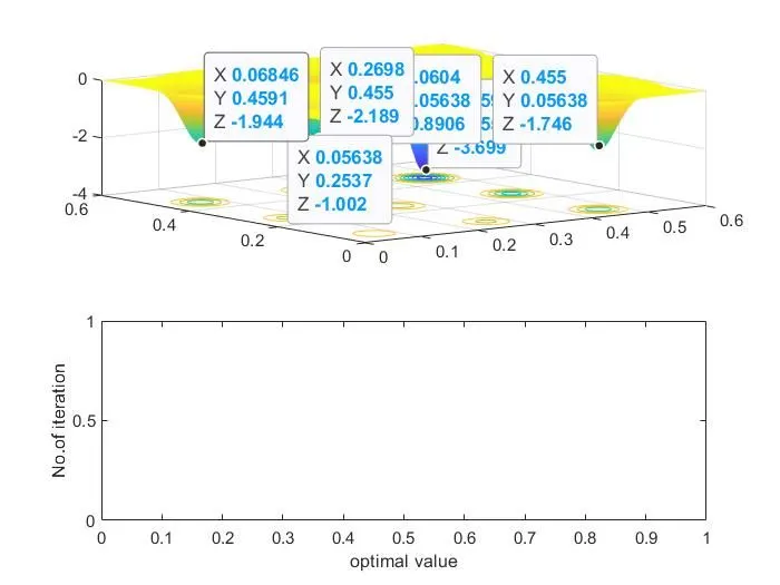
figure(1)
study1_time = toc
subplot(2,1,1)
surfc(x,y,F);
shading interp
hold on
plot3(xopt, yopt, Fopt, 'b')
subplot(2,1,2)
plot(Fopt)
xlabel('optimal value')
ylabel('No.of iteration')

Case2: Genetic Algorthim with upper and lower bound Sampling.

%Defining our search space
x = linspace(0,0.6,150);
y = linspace(0,0.6,150);

%creating a 2Dimensional mesh
[xx yy] = meshgrid(x,y);
n=150;

%Evaluating the stalagmite function
for i = 1:length(xx)
for j = 1:length(yy)
input_vector(1)=xx(i,j);
input_vector(2)=yy(i,j);
F(i,j)=stalagmite(input_vector);
end
end

tic
for i = 1:n
[inputs, Fopt(i)] = ga(@stalagmite,2,[],[],[],[],[0:0],[1:1]);


xopt(i) = inputs(1);
yopt(i) = inputs(2);

end

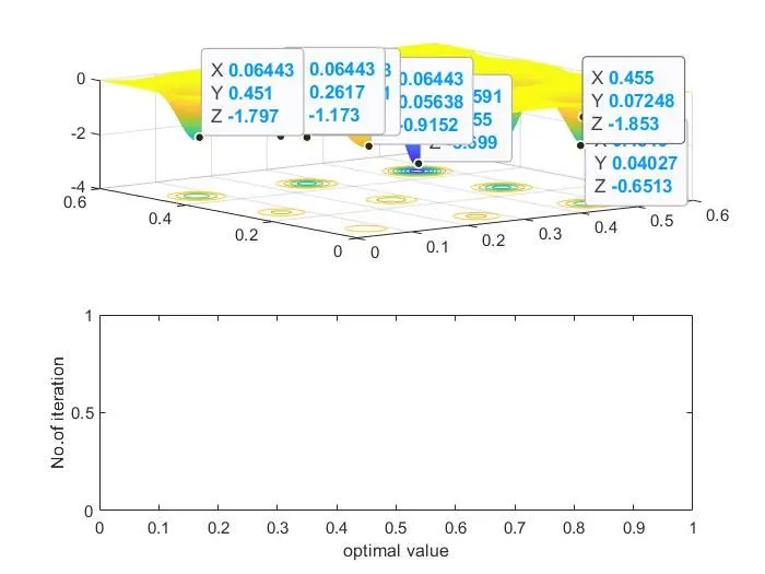
figure(2)
study2_time = toc
subplot(2,1,1)
surfc(x,y,F);
shading interp;
hold on
plot3(xopt, yopt, Fopt,'g');
subplot(2,1,2);
plot(Fopt);
xlabel('optimal value')
ylabel('No.of iteration')

Case3: Genetic Algorthim with upper and lower bound and increase the population size.

%Defining our search space
x = linspace(0,0.6,150);
y = linspace(0,0.6,150);

%creating a 2Dimensional mesh
[xx yy] = meshgrid(x,y);
n=150;

%Evaluating the stalagmite function
for i = 1:length(xx)
for j = 1:length(yy)
input_vector(1)=xx(i,j);
input_vector(2)=yy(i,j);
F(i,j)=stalagmite(input_vector);
end
end

options=optimoptions('ga');
options=optimoptions(options,'populationsize',450);
tic
for i = 1:n
[inputs, Fopt(i)] = ga(@stalagmite,2,[],[],[],[],[0:0],[1:1],[],[],options);


xopt(i) = inputs(1);
yopt(i) = inputs(2);

end

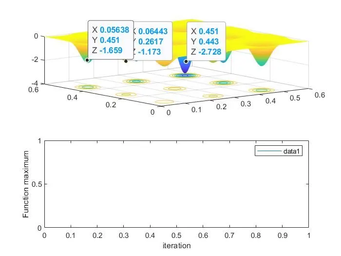
figure(3)
study3_time = toc
subplot(2,1,1)
surfc(x,y,F);
shading interp;
hold on
plot3(xopt, yopt, Fopt,'p');
subplot(2,1,2);
plot(Fopt);
xlabel('iteration')
ylabel('Function maximum');

Code for stalagmiht function:

function f=stalagmite(input_vector)

x=input_vector(1);
y=input_vector(2);

%solving the equations to obtain the values of the function
f1_x = (sin((5.1*pi*x)+0.5))^6;
f1_y = (sin((5.1*pi*y)+0.5))^6;
f2_x = exp(4*log(2)*(((x-0.0667)^2)/0.64));
f2_y = exp(4*log(2)*(((y-0.0667)^2)/0.64));

f = -(f1_x*f1_y*f2_x*f2_y);

end

outputs: