Week 4.1 - Genetic Algorithm

CODE IN MATLAB TO OPTIMIZE STALAGMITE FUNCTION

Aim:- A code in MatLab to optimize the stalagmite function and to find the global maxima of the function.

Objective:-

(1) To evaluate and plot the stalagmite function.

(2) To optimize the stalagmite function using a genetic algorithm.

(3) To find the global maxima of the stalagmite function.

Theory:-

(1) Optimization:-

Optimization is choosing inputs that will result in the best possible outputs or making things the best they can be. Optimization can mean a variety of things from deciding on the most effective allocation of available resources to producing a design with the best characteristics to choosing control variables that will cause a system to behave as desired. Optimization problems often involve words maximize or minimize. Optimization is also useful when there are limits or constraints on the resources involved or boundaries restricting the possible solutions. Let's take a look at a very simple example of an optimization problem given a parabola as shown in the figure.01 choosing X value to get the largest Y value.

Figure.01 parabola: -

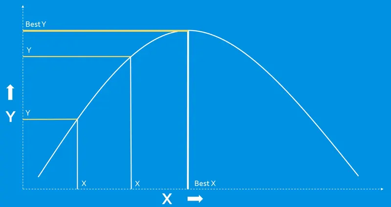
For this simple problem as shown in the figure. 01, it is easy to see the correct solution but for complicated problems it can be difficult to see the correct solution, guessing and checking can take much too long. Hence for such difficult problems, one can use a special type of program which is called an optimization algorithm. Optimization can be applied to a huge variety of situations and problems. For example, choosing the optimal location for a warehouse to minimize shipment times to potential customers, designing a bridge that can carry the maximum load possible for a different cost, designing an airplane wing to minimize weight while maintaining strength. To improve the quality of solutions, if something can be modeled mathematically, it can usually be optimized.

(2) Genetic Algorithm:-

A genetic algorithm is an in-built command in MatLab that minimizes the function by default but an individual can also find the maximum values using the genetic algorithm by converting the function that is to be optimized into a negative function. At the back end of the system, the genetic algorithm works as similar to that of evolutionary techniques discovered by 'Charles Darwin'. It consists of three steps such as selection, crossover, and mutation. Let's understand that how genetic algorithm works behind the scene through the below examples,

Figure.02 Evaluation of initial population: -

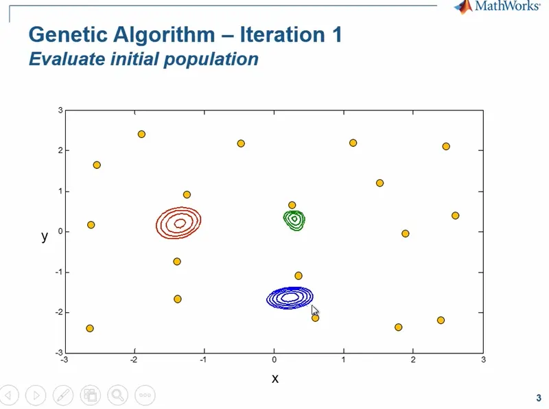
In figure.02, the blue contour represents the global minima point, the red and green contour represents local minima points, and the rest of the orange dots represent initial population points. At first, the genetic algorithm will be going to evaluate all these points and determine the fitness function value for each one of them.

Figure.03 Selection of a few good solutions: -

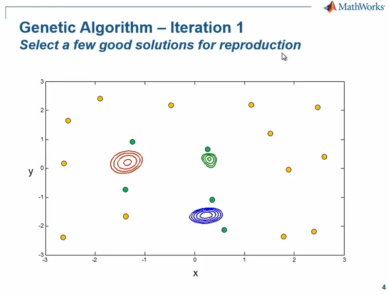
In figure. 03, green dots represent a set of a few good solutions from the initial population for generating a new population.

Figure.04 Generating new population: -

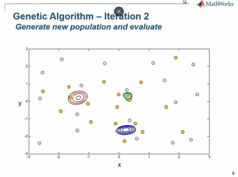
In figure.04, all points represent a set of new population generated through selection, crossover, and mutation. Selection means selecting the best performing points from one generation to the next. Crossover means to generate a child(subsequent generation) based on the common similarities between the parents(inputs variables (x and y)). The mutation is where we take a parent and mutate certain variables to take on random values and we create a child based off of the mutation. The mutation prevents the genetic algorithm to fall into local minima and it really helps it to explore the solution space well.

Figure.05 Evaluation of new population: -

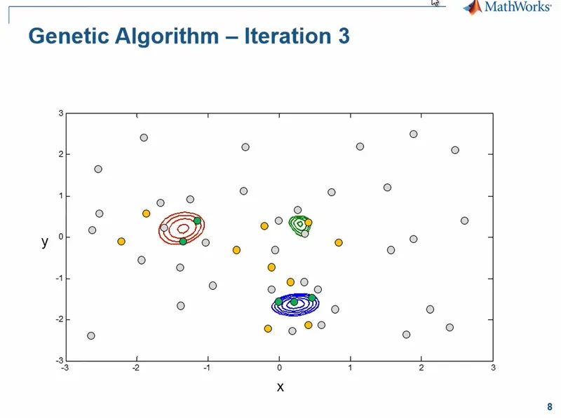
After evaluating the new population shown in the figure. 04, again genetic algorithm will be going to select the few good solutions for next-generation represented by gree dots as shown in the figure. 05.

Figure.06 Converges to the solution: -

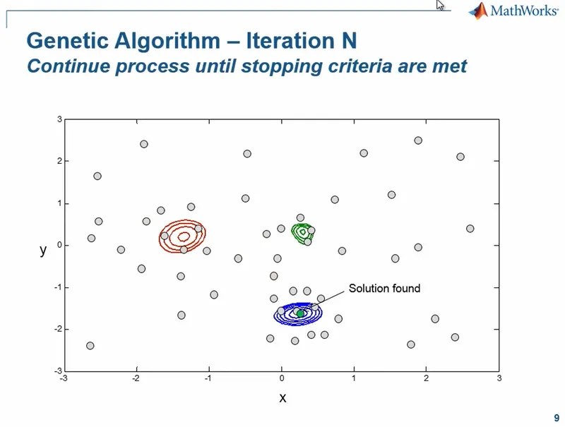
And, it will continue generating new generation one after the other until it converges to a solution as shown in figure.06. The genetic algorithm converges either after hitting a certain number of generations specified or when the best fitness function value is no longer changing or changing to a very small amount.

(3) Stalagmite function:-

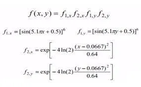
Stalagmite is a mineral deposit found in caves, attached to the grounds as shown in figure.07. Stalagmite is a mathematical function that represents a shape similar to that of stalagmite. A stalagmite function generally refers to the function with which we are generating values over a stalagmite kind of surface for finding out the local and global maxima and minima of that particularly given function.

Figure.07 Stalagmite (mineral deposite): -

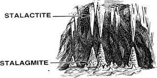
Figure.08 Stalagmite function: -

Program:-

• number '2' in ga(@stalagmite,2) in case 1 part B represents the number of input variables(i.e x and y).
• Four empty square brackets in ga(@stalagmite,2,[],[],[],[],[0;0],[0.6;0.6]) in case 2 part B represents that there are no equations and constraints mentioned for x and y respectively.
• '[0;0],[0.6;0.6]' in ga(@stalagmite,2,[],[],[],[],[0;0],[0.6;0.6]) in case 2 part B represents limits or boundaries for the given function.
• If the population size is not specified in the program then 'ga' will be going to select the first 75 input variables as its 1st set of the initial population by default.

(1) Part A:-

% Part A

% Function
function [f] = stalagmite(input_vector)
f1x = (sin((5.1*pi*input_vector(1))+0.5))^6;
f1y = (sin((5.1*pi*input_vector(2))+0.5))^6;
f2x = exp(-4*log(2)*(((input_vector(1)-0.0667)^2)/0.64));
f2y = exp(-4*log(2)*(((input_vector(2)-0.0667)^2)/0.64));
f = -(f1x*f2x*f1y*f2y);
% -ev sign is to determine global maxima value because genetic algorithm only minimizes the function
end

(2) Part B:-

% Part B

% Optimizing stalagmite function

% Defining search space (Input variables)
x = linspace(0,0.6,500);
y = linspace(0,0.6,500);
% specifying limit(no of interations)
limit = 50;

% Input variables in 2D array
[xx, yy] = meshgrid(x,y);

% Evaluating stalagmite function
for i = 1:length(xx)
    for j = 1:length(yy)
        input_vector(1) = xx(i,j);
        input_vector(2) = yy(i,j);
        f(i,j) = stalagmite(input_vector);
    end
end

% Case 1 (unbounded)

% tic toc command is used to calculate running time
tic
for i = 1:limit
    [input,fval1(i)] = ga(@stalagmite,2);
    x_out1(i) = input(1);
    y_out1(i) = input(2);
end
case_time1 = toc;

% Plots for case 1
figure(1)
subplot(2,1,1)
surfc(xx,yy,-f)
shading interp
hold on
plot3(x_out1,y_out1,-fval1,'marker','o','markersize',5,'markerfacecolor','r')
xlabel('x values')
ylabel('y values')
title('case 1 (unbounded)')
subplot(2,1,2)
plot(-fval1)
xlabel('no of iterations')
ylabel('maximum function values')

% Case 2 (bounded)

% tic toc command is used to calculate running time
tic
for i = 1:limit
    [input,fval2(i)] = ga(@stalagmite,2,[],[],[],[],[0;0],[0.6;0.6]);
    x_out2(i) = input(1);
    y_out2(i) = input(2);
end
case_time2 = toc;

% Plots for case 2
figure(2)
subplot(2,1,1)
surfc(xx,yy,-f)
shading interp
hold on
plot3(x_out2,y_out2,-fval2,'marker','o','markersize',5,'markerfacecolor','r')
xlabel('x values')
ylabel('y values')
title('case 2 (bounded)')
subplot(2,1,2)
plot(-fval2)
xlabel('no of iterations')
ylabel('maximum function values')

% Case 3 (inputting population size)

% for inputting population size
options = optimoptions('ga');
options = optimoptions(options,'populationsize',300);

% tic toc command is used to calculate running time
tic
for i = 1:limit
    [input,fval3(i)] = ga(@stalagmite,2,[],[],[],[],[0;0],[0.6;0.6],[],[],options);
    x_out3(i) = input(1);
    y_out3(i) = input(2);
end
case_time3 = toc;

% Plots for case 3
figure(3)
subplot(2,1,1)
surfc(xx,yy,-f)
shading interp
hold on
plot3(x_out3,y_out3,-fval3,'marker','o','markersize',6,'markerfacecolor','r')
xlabel('x values')
ylabel('y values')
title('case 3 (inputting population size)')
subplot(2,1,2)
plot(-fval3)
xlabel('no of iterations') 
ylabel('maximum function values')

Result:-

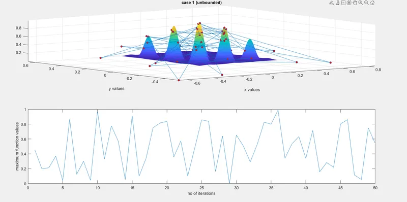
(1) For case 1 (unbounded):-

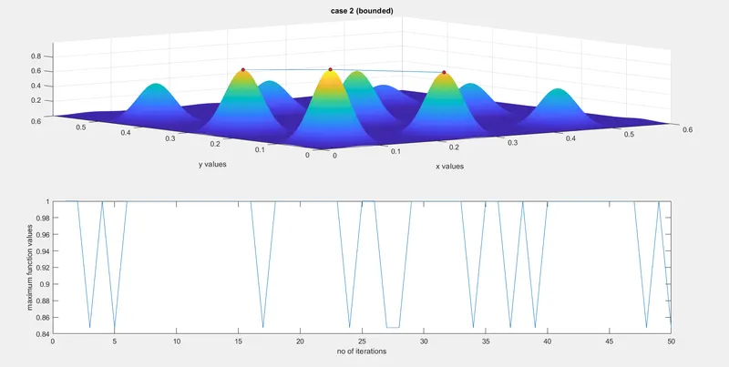
(2) For case 2 (bounded):-

(3) For case 3 (bounded with population size):-

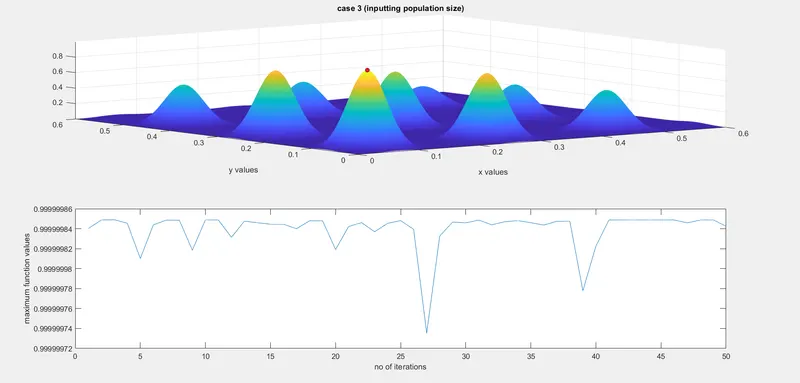
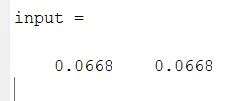
Figure.12 Inputs found in case 3: -

The conclusions from results:-

• From three of the cases, case 3 is the accurate one because in case 3 our 'ga' got converged giving us the global maxima as 1 for the inputs shown in the figure. 12 with very little fluctuation.
• It has been concluded that boundaries or limits and population size are important to get the desired result.
• The more the population size, the more the running time will be.
• We made 'ga' to run 50 times(iterations) in three of the cases in order to check the accuracy(fluctuation) of the results.

Conclusion:-

(1) Optimization becomes easy and efficient through MatLab.

(2) Genetic algorithm in MatLab plays an important role in optimizing problems.

(3) One can easily compare different design points thereby selecting the best design using genetic algorithm techniques in MatLab.