Week 3 - Solving second order ODEs
A Program that solves ODE of Simple Pendulum
Aim:- To write a program that solves 2nd order ordinary differential equation of simple pendulum.
Objective:-
1) To locate the different positions of the oscillating pendulum as a function of time.
2) To study the transient (dependent on time) behavior of the system.
3) To simulate the motion of a simple pendulum on MatLab.
Theory:-
i) Matlab only solves the 1st order ode's. Hence, the first step will be to convert the 2nd order ode into 1st order ode theoretically.
ii) equation of motion (ode) of simple pendulum is written below,
d^2theta/dt^2 + (b/m)*dtheta/dt + (g/l)*sin(theta) = 0
iii)The above ode is determined using Newton's second law of motion.
Calculation:-
1)Conversion of 2nd order ode of simple pendulum into 1st oder ode:-
ode of simple pendulum is,
d^2theta/dt^2 + (b/m)*dtheta/dt + (g/l)*sin(theta) = 0 ...(i)
Assume,
theta = theta1
dtheta/dt = dtheta1/dt = theta2...(a)
d^2theta/dt^2 = d^2theta1/dt^2 = d/dt(dtheta1/dt) = dtheta2/dt
Hence, we get,
theta = theta1...(ii)
dtheta/dt = theta2...(iii)
d^2theta/dt^2 = dtheta2/dt...(iv)
After putting equation no. (ii),(iii) and (iv) in equation no. (i), we get,
dtheta2/dt + (b/m)*theta2 + (g/l)*sin(theta1) = 0 ...(v)
Hence, above equation is the 1st order ode of simple pendulum.
from equation no. (v), we get,
dtheta2/dt = -(b/m)*theta2 - (g/l)*sin(theta1) ...(vi)
& from equation no. (a), we get,
dtheta1/dt = theta2 ...(vii)
Hence, we will be using equation no. (vi) and (vii) to solve ode of simple pendulum in matlab.
Lets write the above values in matrix form,
d/dt[theta1;theta2] = [theta2 ; (-(m/b)*theta2 - (g/l)*sin(theta1))]
note:- (;) is for coloumn matrix.
write [theta1;theta2] as theta, Hence we get,
[dtheta/dt] = [theta2 ; (-(b/m)*theta2 - (g/l)*sin(theta1))] ...(viii)
we'll be using equation no. (viii) format in matlab to solve the given ode.
2)For animation (co-ordinates of the simple pendulum):-
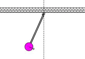
figure.01 animation of a simple pendulum
To animate a simple pendulum as shown in figure.01 in MatLab, there is a need of finding coordinates of each component of a simple pendulum such as hinge support, string, and bob.
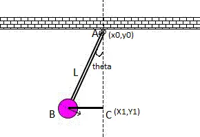
figure.02 oscillating simple pendulum
In the above figure.02,
theta = angular displacement
L = length of the string
If we assume our point A as our origin then (x0,y0) = (0,0)
Hence, co-ordinates for hinge support = (x0,y0) = (0,0)
Since, sin(theta) = opp/hyp = BC/AB = x1/L
Hence, x1 = L*sin(theta)
Since, cos(theta) = adj/hyp = AC/AB = y1/L
Hence, y1 = -L*cos(theta)
Hence, co-ordinates for bob = (x1,y1) = (L*sin(theta),-L*cos(theta))
Coordinates for string will be (x0,y0) = (0,0), (x1,y1) = (L*sin(theta),-L*cos(theta))
Program:-
%part A

%function
function [dtheta_dt] = ode_pendulum(b,g,l,m,theta)
theta1 = theta(1);
theta2 = theta(2);
dtheta1_dt = theta2;
dtheta2_dt = -(b/m)*theta2 - (g/l)*sin(theta1);
dtheta_dt = [dtheta1_dt;dtheta2_dt];
end
%part B
%inputs
%damping co-effient
b = 0.05;
%gravity in m/s^2
g = 9.81;
%length of the string in m
l = 1;
%mass of the bob in kg
m = 1;
%contour (ct)
ct = 1;
%initial conditions, where angular displacement = 0 radian and angular velocity = 3 rad/sec
theta = [0;3];
%time span
t_span = linspace(0,20,25);
%program to solve 2nd order ode of simple pendulum
[t,results] = ode45(@(t,theta) ode_pendulum(b,g,l,m,theta), t_span, theta);
%plot positions of simple pendulum as a function of time
subplot(2,1,1)
%plot for angular displacement
plot(t,results(:,1),'color','r')
%plot for angular velocity
hold on
plot(t,results(:,2),'color','b')
grid on
xlabel('time')
ylabel('plot')
title('time vs plot')
legend('angular displacement','angular velocity')
%for simulating simple pendulum
for i = 1:length(results(:,1))
%co-ordinates of hinge support
x0 = 0;
y0 = 0;
%co-ordiantes of bob
x1 = l*sin(results(i,1));
y1 = -1*cos(results(i,1));
%plot for hinge support
subplot(2,1,2)
plot(x0,y0,'o','markersize',10,'markerfacecolor','g')
%plot for string
hold on
plot([x0 x1],[y0 y1],'linewidth',2,'color','b')
hold on
%plot for bob
plot (x1,y1,'o','markersize',20,'markerfacecolor','r')
grid on
axis([-1.5 1.5 -1.8 1.5]);
pause(0.1);
M(ct) = getframe(gcf);
hold off
ct = ct + 1;
end
%for a movie
movie(M)
videofile = VideoWriter('ode_pendulum.avi','Uncompressed AVI');
open(videofile)
writeVideo(videofile,M)
close(videofile)
Result:-
1)
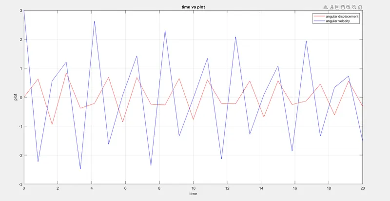
figure.03 time vs plot (angular displacement and angular velocity) graph
2) Video link for an animation of a simple pendulum:-
Conclusion:-
1) Solving ode of a simple pendulum on MatLab, we determined different values of angular displacement (positions) and angular velocity at different time spans easily.
2) Efficiently simulated the simple pendulum on MatLab thereby getting clear visuals.