Project 1 - Parsing NASA thermodynamic data

Parsing Nasa’s Thermodynamic data

Aim: - To parse Nasa’s thermodynamic data file.

Objective: -

1. To write a function to extract 14 coefficients and calculate the specific heat, enthalpy, and entropy for all the species of a data file.
2. To calculate the molecular weight of each species.
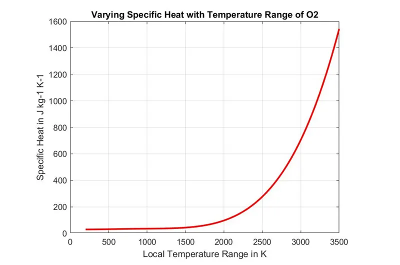
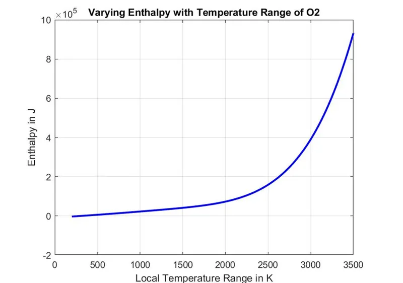
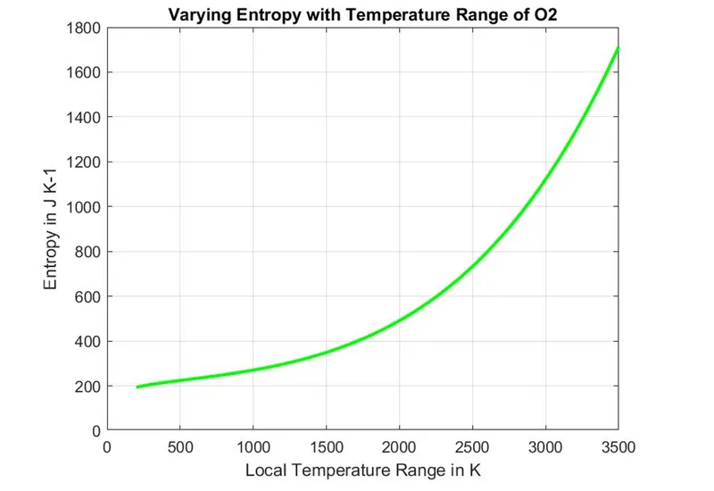
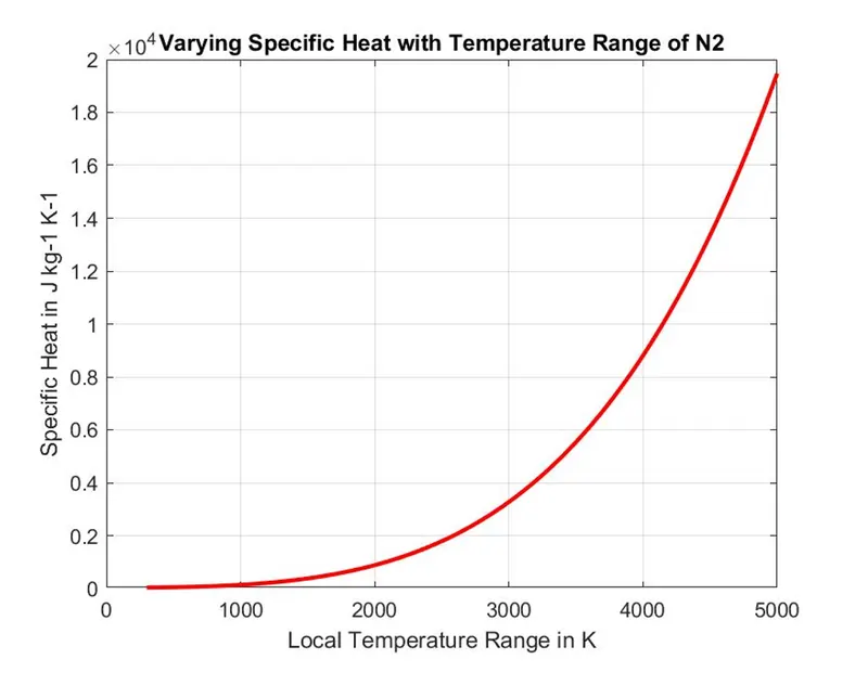
3. To plot specific heat, enthalpy, and entropy with the local temperature range specifically for each species.

Theory: -

1. File parsing: -

We live in a digital world, generating unlimited amounts of data every day. Many users have access to this raw data in different forms such as documents, images, videos, HTML pages, etc. The ability to extract essential information from this data will decide whether we can generate a compelling advantage for our business with this data. However, automating the information extraction process is challenging when dealing with a vast amount of data. Furthermore, as the data accumulation increases, so does the need to read and understand it. This is where the data parsers come into the picture. In simple words, parsing data can help turn unstructured data or unreadable data into more readable and valuable information. We can process data parsing or file parsing using different programming languages such as MatLab, python, java, etc.

2. Common syntaxes for file parsing in MatLab: -

• fopen (filename, permission): - This syntax is used for opening the desired file that had to be parsed. Example no.1.: - In f1 = fopen(‘THERMO.dat’,’r’), f1 is a file handler or a fileID, and the file named as ‘THERMO.dat’ will be open to being parsed using fopen syntax. Here, ‘r’ represents reading of the desired data file.

• fgetl(fileID): - This syntax is used to read or extract the n number of lines from the data file one after the another.

• strsplit (str, delimiter): - This syntax is used to convert a line into a cell array.

• strfind (str, pat): - This syntax is used to find the positions of the desired references.
• str2double (str): - This syntax is used to convert a string into a number.
• fscanf (fileID, formatSpec): - This syntax reads data from an open text file into column vector and interprets value in the file according to the format specified by formatSpec.

• fprintf (formatSpec, A): - This syntax is used to write information or data in a text file.

3. Nasa’s Thermodynamic data: -

Nasa came up with polynomials that can be used to evaluate thermodynamic properties such as specific heat, enthalpy, and entropy. They have also documented the coefficients that are required to evaluate these polynomials for 1000+ species.

(a) Nasa’s Polynomials: -

Thermodynamic properties: -

• Specific heat(cp): -

The specific heat capacity of a substance is the amount of energy required to raise the temperature of 1 kg of the substance by 1-degree celsius.

Formula is given by: -

c = E/m*theta

Where c = specific heat in joules per kg degree Celcius

E = thermal energy in joules

m = mass in kg

theta = temperature in degree celsius

(b) Example of specific heat capacity: -

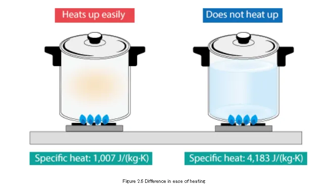
• Enthalpy: -

Enthalpy is the amount of heat content used or released in a system at constant pressure.

It is given by,

H = U + PV

Where H = enthalpy

U = internal energy

P = constant pressure

At constant pressure, heat flow(q) for the processes is equal to the change in enthalpy. It is given by,

deltaH = q

(c) Enthalpy of vaporization: -

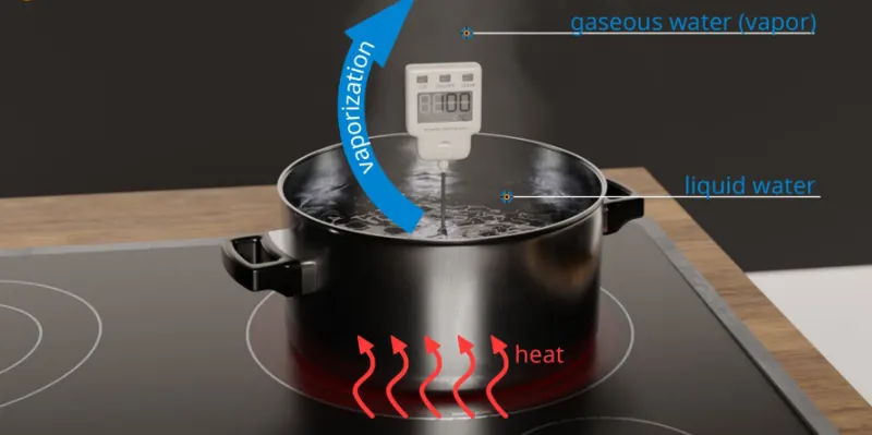
Now, we see an enthalpy change in the vaporization of water. Also, called as enthalpy of vaporization. It is defined as the enthalpy change record to transform the given quantity of a substance from a liquid phase into a gaseous phase at a given pressure. Here, the water system absorbs the heat from the surrounding thereby increasing the heat flow(q) i.e., positive (greater than zero). Hence, deltaH is also positive because of which this reaction is an endothermic reaction.

(d) Dissolution of sodium hydroxide: -

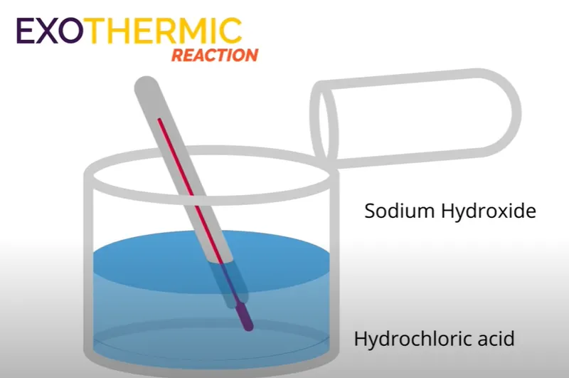
Next, enthalpy change in the dissolution of sodium hydroxide in hydrochloric acid. Sodium hydroxide is dissolved into a sodium ion and hydroxide ion. Heat is released to the surrounding during the dissolution of sodium hydroxide thereby decreasing heat flow(q) i.e., negative (less than zero). Hence, deltaH is also negative because of which this reaction is an exothermic reaction.

• Entropy: -

Work is obtained from ordered molecular motion, the amount of entropy is a measure of the molecular disorder or randomness of a system.

(e) Example of entropy: -

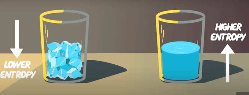
Program: -

• Part A: - Main Program

close all
clc

% Part A

% Universal gas constant in J K-1 mol-1
R = 8.314;

% Reading data file

% Opening data file
f1 = fopen('THERMO.dat','r');

% Skipping first 5 comment lines of data file
for i = 1:5
    get = fgetl(f1);
end

% Extracting next 4 lines of 1st species of data file. Also, extracting the remaining 52 species forming a for loop.
for i = 1:53

    % Starting with the 6th line of data file
    get6 = fgetl(f1);
    % Extracting species name
    line6 = strsplit(get6,' ');
    species_name = line6{1};
    %Extracting local temperatures
    dot = strfind(get6,'.');
    local_low_temp = str2double(get6(dot(1)-3:dot(1)));
    local_mid_temp = str2double(get6(dot(3)-4:dot(3)));
    local_high_temp = str2double(get6(dot(2)-4:dot(2)));
    % Creating local temperature range
    temp = linspace(local_low_temp,local_high_temp,1000);

    % Extracting co-efficients
    % Extracting co-efficients of 7th line
    get7 = fgetl(f1);
    E1 = strfind(get7,'E');
    a1 = str2double(get7(E1(1)-10:E1(1)+3));
    a2 = str2double(get7(E1(2)-11:E1(2)+3));
    a3 = str2double(get7(E1(3)-10:E1(3)+3));
    a4 = str2double(get7(E1(4)-11:E1(4)+3));
    a5 = str2double(get7(E1(5)-10:E1(5)+3));
    % Extracting co-efficients of 8th line
    get8 = fgetl(f1);
    E2 = strfind(get8,'E');
    a6 = str2double(get8(E2(1)-10:E2(1)+3));
    a7 = str2double(get8(E2(2)-10:E2(2)+3));
    a8 = str2double(get8(E2(3)-10:E2(3)+3));
    a9 = str2double(get8(E2(4)-11:E2(4)+3));
    a10 = str2double(get8(E2(5)-10:E2(5)+3));
    % Extracting co-efficients of 9th line
    get9 = fgetl(f1);
    E3 = strfind(get9,'E');
    a11 = str2double(get9(E3(1)-11:E3(1)+3));
    a12 = str2double(get9(E3(2)-10:E3(2)+3));
    a13 = str2double(get9(E3(3)-11:E3(3)+3));
    a14 = str2double(get9(E3(4)-10:E3(4)+3));

    % Calculating specific heat (cp) in J kg-1 K-1
    cp = specific_heat(a1,a2,a3,a4,a5,a8,a9,a10,a11,a12,R,temp,local_mid_temp);

    % Calculating enthalpy (H) in J
    H = enthalpy(a1,a2,a3,a4,a5,a6,a8,a9,a10,a11,a12,a13,R,temp,local_mid_temp);

    % Calculating entropy (S) in J K-1
    S = entropy(a1,a2,a3,a4,a5,a7,a8,a9,a10,a11,a12,a14,R,temp,local_mid_temp);

    % Molecular weight in Kg
    W = molecular_weight(species_name);

    % Making directory for each species
    mkdir(species_name);
    cd(species_name);

    % Plot of Local Temperature Range (temp) Vs Specific Heat (cp)
    figure(1);
    plot(temp,cp,'linewidth',2,'color','r')
    xlabel('Local Temperature Range in K')
    ylabel('Specific Heat in J kg-1 K-1')
    title(sprintf('Varying Specific Heat with Temperature Range of %s',species_name ))
    grid on
    saveas(1,'cp.jpg')

    % Plot of Local Temperature Range (temp) Vs Enthalpy (H)
    figure(2);
    plot(temp,H,'linewidth',2,'color','b')
    xlabel('Local Temperature Range in K')
    ylabel('Enthalpy in J')
    title(sprintf('Varying Enthalpy with Temperature Range of %s',species_name ))
    grid on
    saveas(2,'H.jpg')

    % Plot of Local Temperature Range (temp) Vs Entropy (S)
    figure(3);
    plot(temp,S,'linewidth',2,'color','g')
    xlabel('Local Temperature Range in K')
    ylabel('Entropy in J K-1')
    title(sprintf('Varying Entropy with Temperature Range of %s',species_name ))
    grid on
    saveas(3,'S.jpg')
    
    cd ..
    
end

• Explanation of the main program (of extracting species names, local temperatures, and 14 coefficients): -

• step1: - Opening and reading the text file THERMO.dat using f1 = fopen(‘THERMO.dat’,’r’) syntax. Where, r represents the read command and f1 is a fileID or a file handler.

• step2: - Skipping the first five comment lines of the data file forming a loop using get = fgetl(f1) syntax.

• step3: - Reading line 6 using get6 = fgetl(f1) syntax for extracting species names and local temperatures.

• step4: - Converting line 6 into a cell array using strsplit (get6,’ ‘) syntax.
• step5: - Further, extracting species names using species_names = line {6} syntax.
• step6: - Finding positions of the dot of local temperatures in line 6 using dot = strfind(get6,’.’) syntax.

• step7: - Extracting local low, mid and high temperatures and also converting them from strings into numbers using str2double (get6(dot (1)-3:dot (1))), str2double (get6(dot (3)-4:dot (3))) and str2double (get6(dot (2)-4:dot (2))) syntaxes respectively, taking dots of local temperatures as a reference point.
• step8: - Creating local temperature range using linspace (local_low_temp, local_high_temp,1000) syntax.

• step9: - Next, reading line 7 using get7 = fgetl(f1) syntax for extracting first five coefficients of 1^st species.
• step10: - Finding positions of E in line 7 using E1 = strfind(get7,’E’) syntax.
• step11: - Extracting 1^st co-efficient of 1^st species using a1 = str2double(get7(E1(1)-10: E1(1) +3)) syntax. Similarly, the next 4 coefficients of line 7 of 1^st species will be extracted taking E as a reference.
• step12: - Similarly, the remaining 9 coefficients of 1^st species from lines 8 and 9 will be extracted, taking E as a reference point every time.
• step13: - Form a loop for extracting the remaining 52 species, once the 1^st species is extracted.

• Part B: - Function for calculating Specific Heat

% Part B

% Function for calculating specific heat
function cp = specific_heat(a1,a2,a3,a4,a5,a8,a9,a10,a11,a12,R,T,local_mid_temp)

if T>local_mid_temp
    cp = R*(a1 + (a2.*T) + (a3*(T.^2)) + (a4*(T.^3)) + (a5*(T.^4)));
    % If temperature is greater than local mid temperature then co-effients will be taken from the first seven co-efficients.
else
    cp = R*(a8 + (a9.*T) + (a10*(T.^2)) + (a11*(T.^3)) + (a12*(T.^4)));
    % Else, co-effients will be taken from the second seven co-efficients.
end

end

• Part C: - Function for calculating Enthalpy

% Part C

% Function for calculating enthalpy
function H = enthalpy(a1,a2,a3,a4,a5,a6,a8,a9,a10,a11,a12,a13,R,T,local_mid_temp)

if T>local_mid_temp
    H = R*T.*(a1 + ((a2*T)./2) + ((a3*(T).^2)/3) + ((a4*(T).^3)/4) + ((a5*(T).^4)/5) + a6./T);
    % If temperature is greater than local mid temperature then co-effients will be taken from the first seven co-efficients.
else
    H = R*T.*(a8 + ((a9*T)./2) + ((a10*(T).^2)/3) + ((a11*(T).^3)/4) + ((a12*(T).^4)/5) + a13./T);
    % Else, co-effients will be taken from the second seven co-efficients.
end

end

• Part D: - Function for calculating Entropy

% Part D

% Function for calculating entropy
function S = entropy(a1,a2,a3,a4,a5,a7,a8,a9,a10,a11,a12,a14,R,T,local_mid_temp)

if T>local_mid_temp
    S = R*((a1.*(log(T))) + (a2.*(T)) + ((a3*((T).^2))/2) + ((a4*((T).^2))/3) + ((a5*((T).^4))/4) + a7);
    % If temperature is greater than local mid temperature then co-effients will be taken from the first seven co-efficients.
else
    S = R*((a8.*(log(T))) + (a9.*(T)) + ((a10*((T).^2))/2) + ((a11*((T).^2))/3) + ((a12*((T).^4))/4) + a14);
    % Else, co-effients will be taken from the second seven co-efficients.
end

end

• Part E: - Function for calculating Molecular weight

% Part E

% Function for calculating molecular weight

function W = molecular_weight(species_name)

% Defining 5 main elements atomic names using which all 53 species have formed
atomic_name = ['H','C','O','N','Ar'];

% Defining atomic masses of 5 main elements
atomic_weight = [1.008 12.011 15.999 14.007 39.948];

% Defining starting range of molecular weight
W = 0;

% forloop for calculating atomic weight of each species
for i = 1:length(species_name)
    for j = 1:length(atomic_name)
        if strcmp(species_name(i),atomic_name(j))
            W = W + atomic_weight(j);
            position = j;
        end
    end
    % Checking other elements in species
    n = str2double(species_name(i));
    if n>1
        W = W + atomic_weight(position)*(n-1);
    else

    end
end

% Displaying molecular weight in command window

fprintf('molecular weight of %s :-  ',species_name);
fprintf('%f',W);
disp(' ');

end

• Working of molecular weight program: -

• Let's take an example of species C3H8 for understanding the back-end scenario for calculating the molecular weight for each species. Species C3H8 is divided into 4 parts while solving in Matlab.
• Once the program is executed, MatLab will first calculate the molecular weight for C(1st part) which is 12.011.
• Next, for number 3(2nd part) in the formula, it is clearly mentioned in the program that if other elements(n) are greater than 1 then the main formula will be multiplied by (n-1).
• Since number 3 is greater than 1, MatLab will put the molecular weight of C calculated in place of molecular starting range(W) and also in place of atomic weight multiplying it with (3-1) shown as: - W = 12.011+12.011*(3-1).
• The recent answer for molecular weight is now 36.033.
• For H(3rd part), MatLab will put recent molecular weight in place of molecular starting range(W) and 1.008(molecular weight of H) in place of atomic weight shown as: - W = 36.033 + 1.008.
• The recent answer for molecular weight is now 37.041.
• Since number 8(4th part) is greater than 1, MatLab will put the recent molecular weight calculated in place of molecular starting range(W) and 1.008(molecular weight of H) in place of atomic weight multiplying it with (8-1) shown as- W = 37.041+1.008*(8-1).
• After solving all parts of species, the final molecular weight of species C3H8 is 44.097.

Result: -

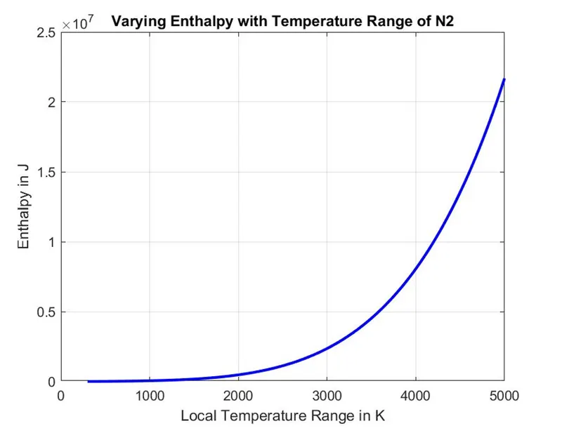
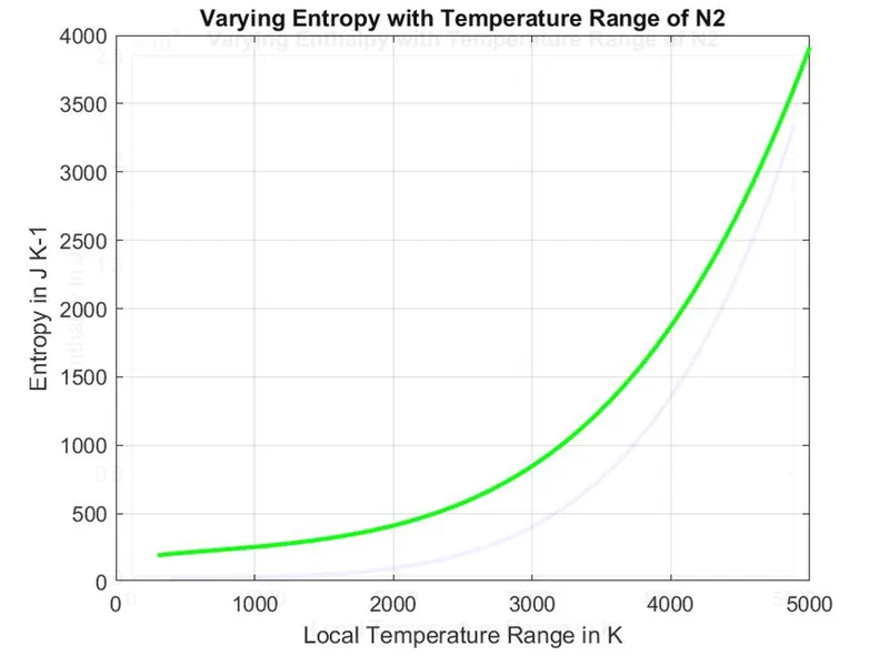
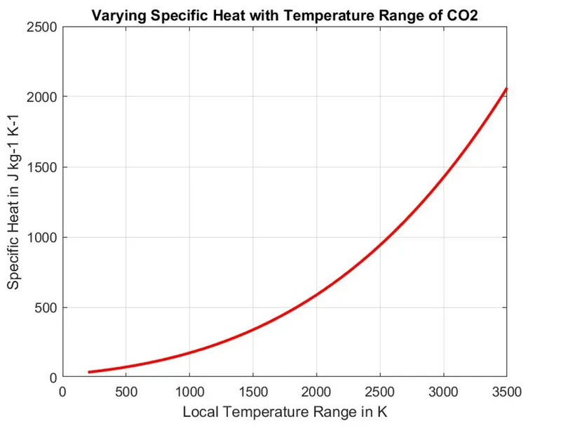
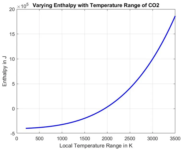
• Plots of specific heat, enthalpy, and entropy for local temperature range for O2, N2, and CO2.

• Plots of O2: -

• Plots of N2: -

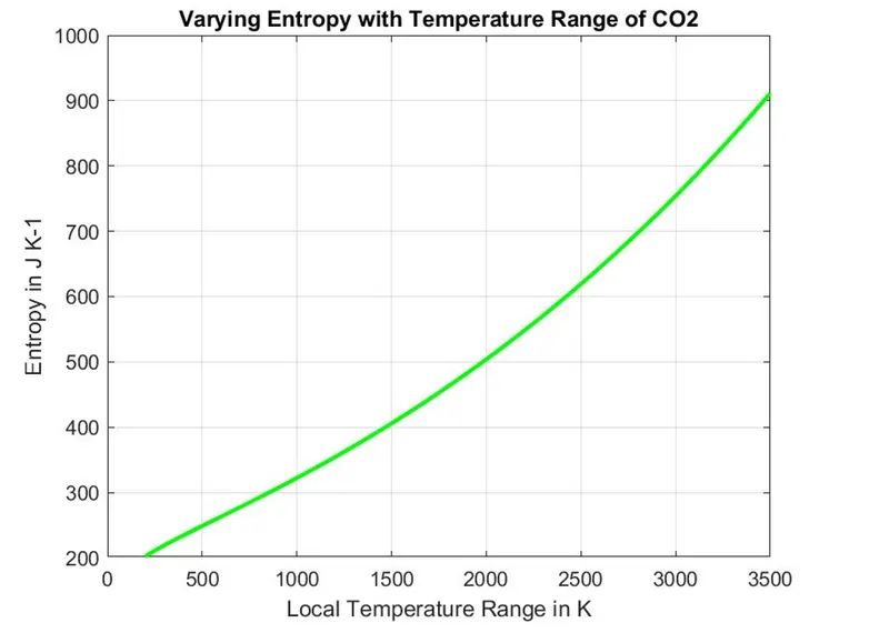
• Plots of CO2: -

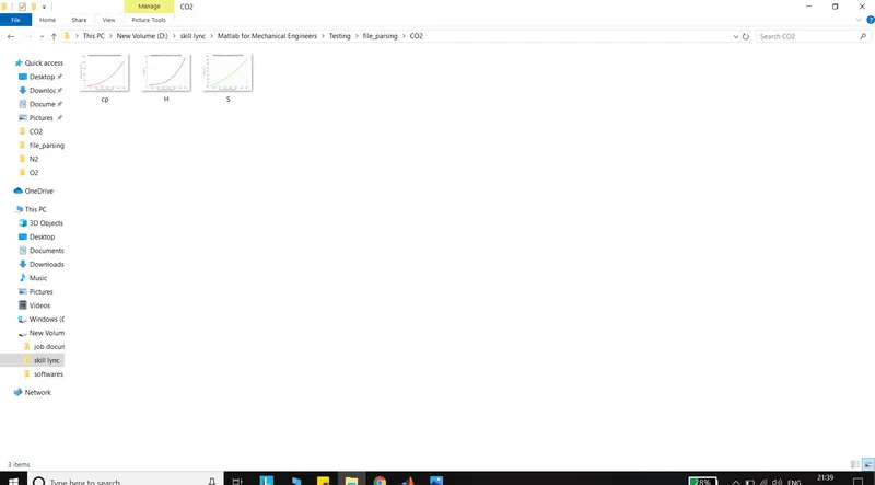
• folders in which O2, N2, and CO2 plots are saved: -

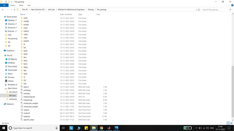
• folders where all plots are saved: -

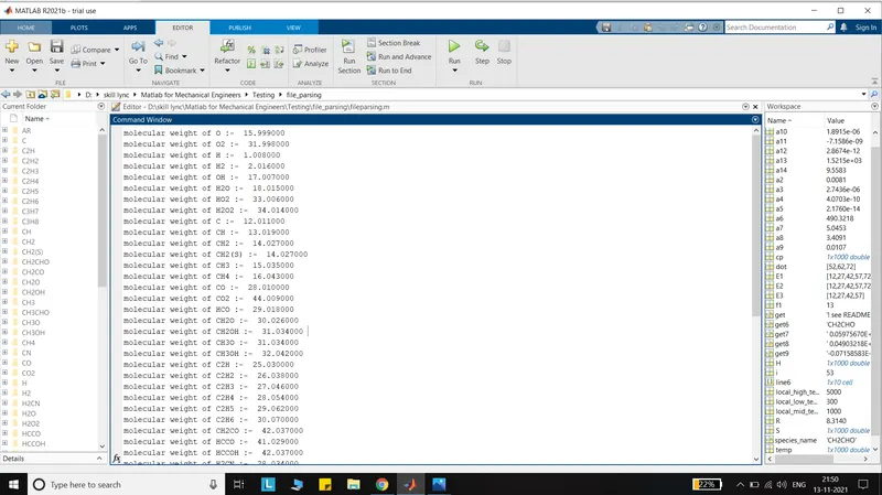
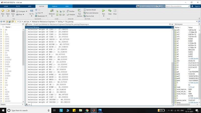
• Display of molecular weights for each species in the command window: -

Conclusion: -

• File parsing results in the eradication of repetitive data entry.
• It also removes data processing errors.
• It can lead to an increase in employee productivity.
• It supports in Automatic fulfillment of company or industry compliance procedures.
• It helps in Hassle-free data transferring.