Week 4.1 - Genetic Algorithm
AIM : To write a code using MATLAB to optimise the stalagmite function, find the global maxima of the function and plot the graph.
OBJECTIVE :
- To write a code using MATLAB to optimise the stalagmite function.
- Find the global maxima of the function.
- Explain the concept of genetic algorithm and also explain the syntax for ga in MATLAB.
- Plot graphs for all 3 studies and for F maximum vs no. of iterations.
THEORY :
Optimisation :
Optimisation is a decision making process, it helps to find the best results, under a set of prioritized criteria or constraints. It is a procedure which is executed iteratively by comparing various solutions till an optimum or a satisfactory solution is found.
In the simplest case, an optimization problem consists of maximizing or minimizing a real function by systematically choosing input values from within an allowed set and computing the value of the function. The generalisation of optimisation theory and techniques to other formulations constitutes a large area of applied mathematics. More generally, optimisation includes finding "best available" values of some objective function given a defined domain (or input), including a variety of different types of objective functions and different types of domains.
Genetic Algorithm :
A genetic algorithm is a search heuristic that is inspired by Charles Darwin's theory of natural evolution. This algorithm reflects the process of natural selection where the fittest individuals are selected for reproduction in order to produce offspring of the next generation.
In simple words Genetic Algorithm is a search-based optimisation technique based on the principles of Genetics and Natural Selection. It is frequently used to find optimal or near-optimal solutions. It is used to solve optimisation problems, in research, and in machine learning.
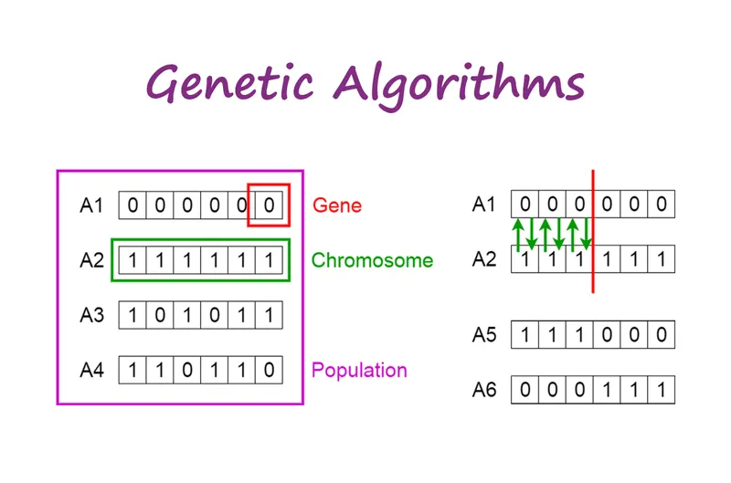
Five phases are considered in a genetic algorithm.
1. Initial population
2. Fitness assignment
3. Selection
4. Crossover
5. Mutation
1. Initial Population :
- The process begins with a set of individuals which is called a Population. Each individual is a solution to the problem you want to solve .
- An individual is characterized by a set of parameters (variables) known as Genes. Genes are joined into a string to form a Chromosome (solution).
- In a genetic algorithm, the set of genes of an individual is represented using a string, in terms of an alphabet. Usually, binary values are used (string of 1s and Os). We say that we encode the genes in a chromosome
2. Fitness assignment :
The fitness assignment determines how fit an individual is (the ability of an individual to compete with other individuals). It gives a fitness score to each individual. The probability that an individual will be selected for reproduction is based on its fitness score.
3. Selection :
- The idea of the selection phase is to select the fittest individuals and let them pass their genes to the next generation.
- Two pairs of individuals selected for reproduction are selected based on their fitness scores. Individuals with high fitness have more chances to be selected for reproduction.
4. Crossover :
Crossover is the most significant phase in a genetic algorithm. For each pair of parents to be mated, a crossover point is chosen at random from within the genes.
5. Mutation:
In certain new offspring formed, some of their genes can be subjected to a mutation with a low random probability. This implies that some of the bits in the bit string can be flipped.
The following flow chart describes how the genetic algorithm works to find the optimal solution.
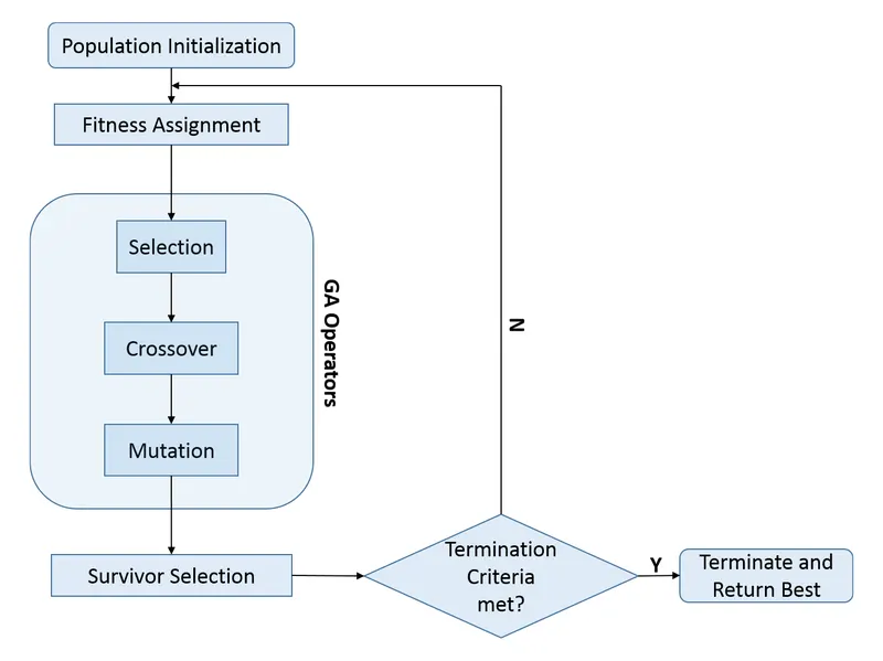
The following outline summarizes how the genetic algorithm works :
1. The algorithm begins by creating a random initial population.
2. The algorithm then creates a sequence of new populations. At each step, the algorithm uses the individuals in the current generation to create the next population. To create the new population, the algorithm performs the following steps:
- Scores each member of the current population by computing its fitness value. These values are called the raw fitness scores.
- Scales the raw fitness scores to convert them into a more usable range of values. These scaled values are called expectation values.
- Selects members, called parents, based on their expectation.
- Some of the individuals in the current population that have lower fitness are chosen as elite. These elite individuals are passed to the next population.
- Produces children from the parents. Children are produced either by making random changes to a single parent-mutation-or by combining the vector entries of a pair of parents-crossover.
- Replaces the current population with the children to form the next generation.
3. The algorithm stops when one of the stopping criteria is met.
The termination condition of a Genetic Algorithm is important in determining when a GA run will end. It has been observed that, initially, the GA progresses very fast with better solutions coming in every few iterations, but this tends to saturate in the later stages where the improvements are very small. We usually want a termination condition such that our solution is close to the optimal, at the end of the run.
Stoping Criteria :
Usually, we keep one of the following termination conditions -
- When there has been no improvement in the population for X-number of generations.
- When we reach an absolute number of generations.
- When the objective function value has reached a certain predefined value.
Application of genetic algorithm :
Genetic Algorithms are primarily used in optimization problems of various kinds, but they are frequently used in other application areas as well.
The areas in which Genetic Algorithms are frequently used are listed below.
- Optimization :- Genetic Algorithms are most commonly used in optimization problems wherein we have to maximize or minimize a given objective function value under a given set of constraints.
- Economics :- GAs are also used to characterize various economic models like the cobweb model, game theory equilibrium resolution, asset pricing, etc.
- Neural Networks :- GAs are also used to train neural networks, particularly recurrent neural networks.
- Image Processing :- GAs are used for various digital image processing (DIP) tasks as well like dense pixel matching.
Syntax for Genetic algorithm(ga) :
- For random inputs :
x = ga(fun,nvars) finds a local unconstrained minimum, x, to the objective function, fun,nvars is the dimension (number of design variables) of fun.
- For bounded inputs :
x = ga(fun,nvars,A,b) finds a local minimum x to fun, subject to the linear inequalities `Axxx<=b`. ga evaluates the matrix product A*x as if x is transposed (A*x).
x = ga(fun,nvars,A,b,`A_(eq),b_(eq)`) finds a local minimum x to fun, subject to the linear equalities `A_(eq)xxx= b_(eq) and Axxx<=b` (Set A=[ ] and b=[ ] if no linear inequalities exist.) ga evaluates the matrix product `A_(eq)xxx` as if x is transposed (`A_(eq)xxx`).
x = ga(fun,nvars,A,b,`A_(eq) ,b_(eq)`,lb,ub,nonlcon) subjects the minimization to the constraints defined in nonlcon. The function nonlcon accepts x and returns vectors C and `C_(eq)`, representing the nonlinear inequalities and equalities respectively. ga minimizes the fun such that C(x) ≤ 0 and `C_(eq)`(x) = 0. (Set lb=[ ] and ub=[ ] if no bounds exist.)
- For Population size :
x=ga(fun,nvars,A,b,`A_(eq) ,b_(eq)`,lb,ub,nonlcon,intcon,options) requires that the variables listed in IntCon take integer values.
optimoptions(SolverName,Name,Value)
This command is used to give options to ga.Its take the solver name,name of the options and value as inputs.
Where,
fun = function,
nvars = Number of Variables
A = Linear inequality constraints
b = Linear inequality constraints
`A_(eq)` = linear equality constraints
`b_(eq)` = linear equality constraints
lb = lower Bounds.
ub = Upper Bounds
nonIcon = Non-Linear Constraints
intcon = Integer Constraints
GOVERNING EQUATIONS :
Stalagmite Function :
A stalagmite function generally refers to the function with which we are generating values over a stalagmite kind of surface for finding out the local and global maxima and minima of that particular given function.
The given stalagmite function is,
`f(x,y) = f_(1x)*f_(2x)*f_(1y)*f_(2y)`
where,
`f_(1x) = [sin(5.1pix+0.5)]^6`
`f_(1y) = [sin(5.1piy+0.5)]^6`
`f_(2x) = exp[-4ln(2)(x-0.0667)^2/0.64]`
`f_(2y) = exp[-4ln(2)(y-0.0667)^2/0.64]`
MATLAB CODE :
Program 1 : The Stalagmite function.
- The Stalagmite function is a core part of the code.
- The function follows the formula stated in the Equations Used.
- The 'Function' input is used to write a function code.
function [F] = stalagmite(input_vectors)
a = input_vectors(1);
b = input_vectors(2);

% calculating the term in the function

f1x = (sin(5.1*pi*a+0.5)).^6;
f1y = (sin(5.1*pi*b+0.5)).^6;

f2x = exp(-4*log(2)*((a-0.0667).^2/0.64));
f2y = exp(-4*log(2)*((b-0.0667).^2/0.64));

F = -(f1x.*f1y.*f2x.*f2y);          % Negative sign is used to calculate the global maxima
end
Program 2 : Evoluating the stalagmite function and to write the code for unbounded inputs,bounded inputs and bounded inputs with increase in population.
clear all
close all
clc

% Inputs

x = linspace(0,0.6,150);
y = linspace(0,0.6,150);

% Creating a matrix of 2x2

[xx,yy] = meshgrid(x,y);

% Evaluating the stalagmite function

for i = 1:length(xx)
    for j =1: length(yy)
        input_vectors(1) = xx(i,j);
        input_vectors(2) = yy(i,j);
        F(i,j) = stalagmite(input_vectors);
    end
end

% Study_1 for unbounded inputs

num_counts = 50;              % Iteration counts
tic                           % start the clock time for function

for i = 1:num_counts
    [inputs, fopt(i)] = ga(@stalagmite,2);
    xopt(i) = inputs(1);
    yopt(i) = inputs(2);
end

studytime_1 = toc             % calculating time for the function execution

figure(1)
subplot(2,1,1)
hold on
surfc(x,y,-F)

shading interp
xlabel('X-axis')
ylabel('Y-axis')
plot3(xopt,yopt,-fopt,'marker','o','markersize',5,'markerfacecolor','r')

title('Unbounded inputs')
subplot(2,1,2)

plot(-fopt)
xlabel('Iteration')
ylabel('Function maximum')

% Study_2 for bounded inputs

tic                           % start the clock time for function

for i = 1:num_counts
    [inputs, fopt(i)] = ga(@stalagmite,2,[],[],[],[],[0;0],[0.3;0.3]);
    xopt(i) = inputs(1);
    yopt(i) = inputs(2);
end

studytime_2 = toc             % calculating time for the function execution

figure(2)
subplot(2,1,1)
hold on
surfc(x,y,-F)

shading interp
xlabel('X-axis')
ylabel('Y-axis')
plot3(xopt,yopt,-fopt,'marker','o','markersize',5,'markerfacecolor','r')

title('bounded inputs')
subplot(2,1,2)

plot(-fopt)
xlabel('Iteration')
ylabel('Function maximum')


% Bounded inputs with population increased

options = optimoptions(@ga);
options = optimoptions(@ga,'populationsize',200);

tic                           % start the clock time for function

for i = 1:num_counts
    [inputs, fopt(i)] = ga(@stalagmite,2,[],[],[],[],[0;0],[0.3;0.3],[],[],options);
    xopt(i) = inputs(1);
    yopt(i) = inputs(2);
end

studytime_3 = toc             % calculating time for the function execution

figure(3)
subplot(2,1,1)
hold on
surfc(x,y,-F)

shading interp
xlabel('X-axis')
ylabel('Y-axis')
plot3(xopt,yopt,-fopt,'marker','o','markersize',5,'markerfacecolor','r')

title('Bounded inputs with increased population')
subplot(2,1,2)

plot(-fopt)
xlabel('Iteration')
ylabel('Function maximum')
Step wise explanation of the code :
For Program 1 :
- The code is used to get the value of the function (F) at different grid points on the x-y plane which will be plotted in the z-direction.
- Created an variable a and b to stored the given input parameters.
- The stagalmite function and the equation were created using variables `f_(1x),f_(1y),f_(2x) and f_(2y)`.
- we have multiplied the -ve sign to convert the function into maxima since the genetic algorithm function can only calcualte the minima value for a function.
For Program 2 :
1. The code starts with the command clear all, close all and clc. Where,
- clear all : it is used to clear the data stored in workspace.
- close all : it is used to close all the plots abd figure.
- clc : it is used to clear the command window.
2. First, the inputs for defining the workspace are given. It is given using the linspace command. The values are stored in variables x and y.
3. A 2-D matrix of the same is created using the meshgrid command. It is then stored in arrays xx and yy.
4. Then the value for the stalagmite function is found by with the help of two for loops. The loop counter variables for the loops are i and j. They start from 1 and go up to the length of xx and yy respectively.
5. Then the value of the stalagmite function is computed by calling the function. The formula for the stalagmite function is created in a separate MATLAB function 'stalagmite'.
6. In the first study we have no bounds for the inputs. The population is set as 150.
7. We find the global maximum by giving input as the function and number of design variables.
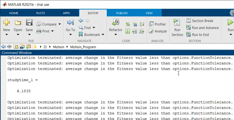
8. The time taken for this computation is calculated by using the tic and toc commands. It is stored in the variable studytime_1.
9. Then, we create a figure window and create a surface plot in it. The local maxima are also plot in the surface plot.
10. The surface plot is made in the figure window 1 as a subplot. In another subplot, we plot the function maximum versus No. of Iterations.
11. In the second study, we calculate the global maxima by giving upper and lower bounds along with the function and no. of design variables.
12. The population is maintained as 150.
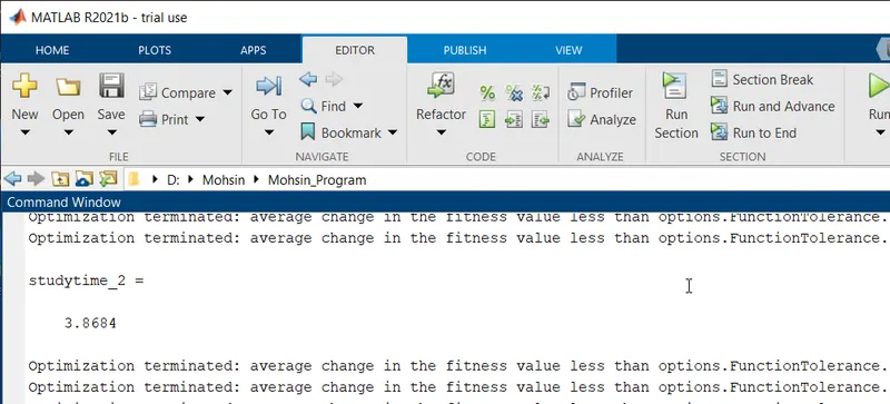
13. As in the previous case, the time taken to compute is calculated with the help of tic and toc commands. The time is stored in the variable studytime_2.
14. Once the global maxima is calculated, we do the plots as in the previous study. For this study, we do the plots in a separate figure window.
15. Finally, in the third study we calculate the global maxima by giving the same upper & lower bounds but with an increased population.
16. In this case. the population is set as 200.
17. As in previous studies, the time for computation is calculated using tic and toc commands and stored in the variable studytime_3.
18. For this purpose, we use the optimoptions command. It enables us to change the default population of 150 and implements this population change in the ga.
19. The plots are plot using the plot command as in the previous cases.
ERRORS FACED WHILE PROGRAMMING :
- The stalagmite function `f_(1x) and f_(1y)` were type error.
Solution: Error is removed by assigning the a and b variable at right place.
- In the for loop for variable j the equation is incorrect due to typo.
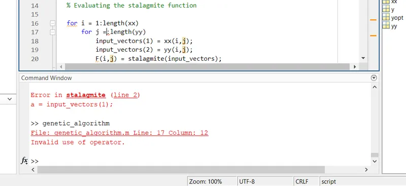
Solution: The error is correct by giving the proper value in line 17 as for = 1:length(yy).
RESULTS :
For Study 1 :
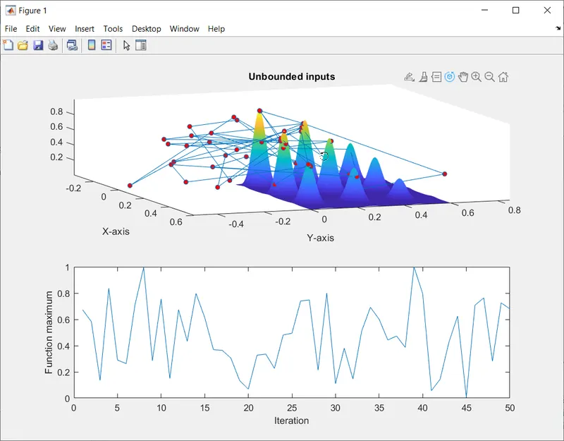
The results obtained for the unbounded inputs vary over a large sized interval. Thus, providing a vague idea of the global maxima. But it can be observed that the value of 'F MAXIMUM' lies between the interval [0, 1]. Therefore, we can opt for bounded inputs that can give more precise results.
For Study 2 :
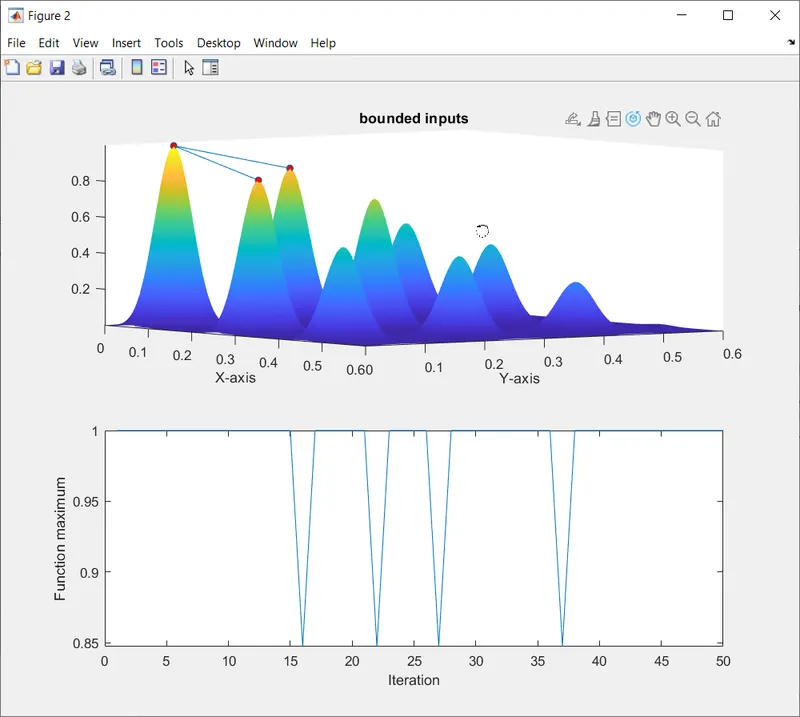
The above graph is more clear and optimised compared to the 1st iteration since here the bounds were defined and we could get only the values within our range. We are now more clear on the range within which our maxima lies.
For Study 3 :
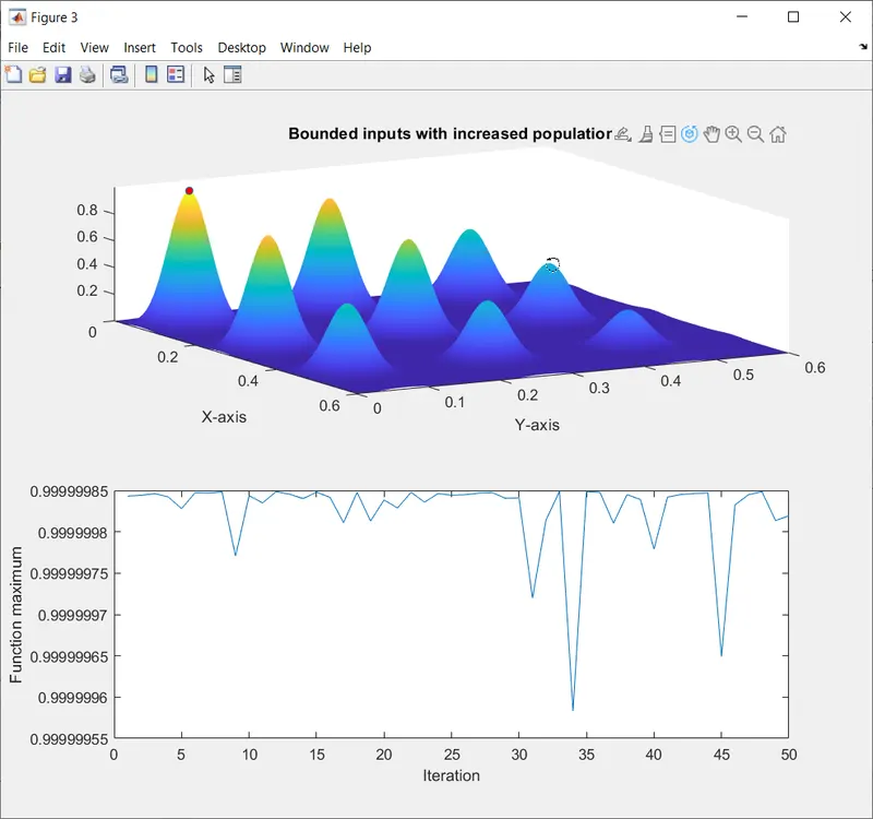
In the third surface plot, we can see that we have obtained the exact global maxima for the function. We only have one point marked, which is the global maxima.
Even in 2-D the, the changes are very less. It indicates we have reached to an optimum point.
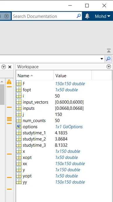
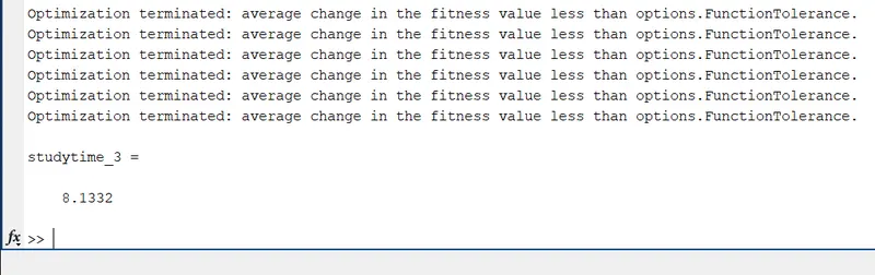
From the output obtained we can see that the time taken for each study process to be more than previous one.
The value for GLOBAL MAXIMA comes out to be at 0.9999996
CONCLUSION :
- Thus the genetic algorithm was used to solve the stalagmite function to optimize the function and find the global maxima. The output surface and 2-D plots obtained are shown.
- The time taken for each study is also recorded and obtained in the workspace.
- We can conclude that by increasing the number of iterations, population and setting lower and upper bounds, we obtain the result for global maxima accurately.
REFERNCES :