Solving second order ODEs

AIM : To create a program in MATLAB to solve and simulate the second order ODE that represent the equation of motion of a simple pendulum with damping.

OBJECTIVE :

• To write a program in MATLAB to solve the second order ODE which represent the equation of motion of a simple pendulum.
• To create an animation of the motion of simple pendulum using MATLAB.

THEORY :

Simple Pendulum :

A simple pendulum is a mechanical arrangement that demonstrates periodic motion. The simple pendulum comprises a small bob of mass ‘m’ suspended by a thin string secured to a platform at its upper end of length L. The simple pendulum is a mechanical system that sways or moves in an oscillatory motion. This motion occurs in a vertical plane and is mainly driven by the gravitational force.

Interestingly, the bob that is suspended at the end of a thread very light somewhat we can say it is even massless. The period of a simple pendulum can be made extended by increasing the length string while taking the measurements from the point of suspension to the middle of the bob. However, it should be noted that if the mass of the bob is changed it will the period remains unchanged. Period is influenced mainly by the position of the pendulum in relation to Earth as the strength of gravitational field is not uniform everywhere.

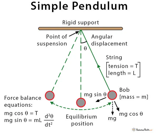
In general the motion of simple pendulam is considered to be simple harmonic motion with constant amplitude and is given by equation;

`(d^2theta)/dt^2 + g/L(sintheta) = 0`

where,

`theta` = angular displacement of the pendulum bob,

g = acceleration due to gravity in `m/s^2`,

L = length of pendulum in m.

In practice the motion of simple pendulum is subjected to a restoring force with friction and air drag which reduces their amplitude of swing with time and bring it back towards the equilibrium position.

When the motion of an oscillator reduces due to an external force, the oscillator and its motion are said to be damped. These periodic motions of gradually decreasing amplitude are damped simple harmonic motion.

The differential equation for the motion of a simple pendulum with damping is as follows,

`(d^2theta)/dt^2 + b/m((d theta)/dt) + g/L(sintheta) = 0`

where,

b = damping coefficient,

m = mass of pendulum in kg.

Ordinary Differential Equation :

An ordinary differential equation (also abbreviated as ODE), in Mathematics, is an equation which consists of one or more functions of one independent variable along with their derivatives. A differential equation is an equation that contains a function with one or more derivatives. But in the case ODE, the word ordinary is used for derivative of the functions for the single independent variable. In case of other types of differential equations, it is possible to have derivatives for functions more than one variable. The types of DEs are partial differential equation, linear and non-linear differential equations, homogeneous and non-homogeneous differential equation.

The order of ordinary differential equations is defined to be the order of the highest derivative that occurs in the equation.

ODEs has remarkable applications and it has the ability to predict the world around us. It is used in a variety of disciplines like biology, economics, physics, chemistry and engineering. It helps to predict the exponential growth and decay, population and species growth. Some of the uses of ODEs are:

• Modelling the growth of diseases
• Describes the movement of electricity
• Describes the motion of the pendulum, waves
• Used in Newton’s second law of motion and Law of cooling

GOVERNING EQUATION :

The differential equation for the motion of a simple pendulum with damping is as follows,

`(d^2theta)/dt^2 + b/m((d theta)/dt) + g/L(sintheta) = 0` ____________ Equation (1).

To solve the above equation in MATLAB, we need to transform the given second order ODE into first ODE as,

`=>` `theta = theta_1`,

`=> (d(theta))/dt = (d(theta_1))/dt = theta_2`,

`=>` `(d^2theta)/dt^2 = (d^2theta_1)/dt^2 = d/dt((d(theta_1))/dt) = (d(theta_2))/dt` __________________ Equation (2),

From Equation (1)

`=> (d^2(theta))/dt^2 + (b/m).((d(theta))/dt) + (g/L).sintheta = 0`

Using Equation (2),

`=> (d^2theta_1)/dt^2 + (b/m).(d(theta_1))/dt + (g/L).sintheta_1 = 0,`

`=> (d(theta_2))/dt + (b/m).(theta_2)+ (g/L).sintheta_1 = 0`,

`=> (d(theta_2))/dt =-(b/m).(theta_2) - (g/L).sintheta_1` ,

The above equation in matrix form,

`d/dt[[theta_1],[theta_2]] = [[theta_2],[[-b/m.theta_2,-g/L.sintheta_1]]]`

where,

`theta_1` = Angular displacement of Pendulum bob,

`theta_2` = Angular velocity of Pendulum bob,

MATLAB CODE :

1. First a function is need to declares where we will define the second order ODE into single order.
2. This function [dtheta_dt] was named as ode_functioon.

Program 1 :

function [dtheta_dt] = ode_function(t,theta,b,g,L,m)

theta1 = theta(1);
theta2 = theta(2);
dtheta1_dt = theta(2);
dtheta2_dt = -(b/m)*theta2 - (g/L)*sin(theta1);
dtheta_dt = [dtheta1_dt;dtheta2_dt];

end

So we need a program to call this function[dtheta_dt] to determine the angular displacement and angular velocity. Also create an animation to show the damping effect on simple pendulum.

Program 2 :

clear all 
close all
clc

% Input Variables
b = 0.05;            % damping coefficient
g = 9.81;            % gravity in (m/s^2)
L = 1;               % length of pendulam
m = 1;               % mass of pendulam in kg

% Initial Condition

theta_0 = [0 ; 3];      % initial  angular displacement and angular Velocity

% Time Points

time_span = linspace(0,20,500);

% To solve ODE

[t, result] = ode45(@(t,theta) ode_function(t,theta,b,g,L,m), time_span, theta_0);

% Plotting angular displacement and angular velocity with respect to time

figure(1)
plot(t,result(:,1),'LineWidth',2);
hold on
plot(t,result(:,2),'LineWidth',2);
axis([0 20 -4 4]);
xlabel('Time in second');
ylabel('Angular displacement and Angular Velocity');
grid on 
title(' Damping effect on Pendulam')
legend('Angular displacement','Angular velocity');

angle = result(:,1);
pause(5);

% counter is used to represent each frame
ct = 1;

for i = 1:length(time_span);

    % fixed co-ordinate of one end of Simple Pendulam

    x0 = 0;
    y0 = 0;

    % Moving co-ordinate of one end of Simple Pendulam

    x_end = L*sin(result(i,1));
    y_end = -L*cos(result(i,1));


    % Simulation of the motion of a pendulam

    figure(2)
    plot([-1 1],[0 0],'LineWidth',6,'color','k');
    hold on
    plot([0 0],[-1.2 0.5],'LineStyle','--','Color','black');
    axis([-1.5 1.5 -1.5 1]);
    line([x0 x_end],[y0 y_end],'LineWidth',2,'color','b');
    plot(x0,y0,'Marker','o','MarkerSize',3,'MarkerFaceColor','r');
    plot(x_end,y_end,'Marker','o','MarkerSize',20,'MarkerFaceColor','r');
    grid on
    title(' Damping effect on Simple Pendulam');
    legend('Support of Pendulam', 'Axis of oscillation','Length of Pendulam', 'Fixed point', 'Bob of Pendulam');
    xlabel('x-axis');
    ylabel('y-axis')
    pause(0.01)
    M(ct) = getframe(gcf);
    ct = ct+1;
    hold off
end

% Animation of the motion of a pendulam

movie(M)
videofile = VideoWriter('Simple_Pendulam.avi','Uncompressed AVI')
open(videofile)
writeVideo(videofile,M)
close(videofile)

Step wise explanation of the code :

1. The code starts with the command clear all, close all and clc. Where,

• clear all : it is used to clear the data stored in workspace.
• close all : it is used to close all the plots abd figure.
• clc : it is used to clear the command window.

2. Now, inputs the given value of gravity, length of the pendulum, mass of the pendulum bob and damping coefficient in the variables g,L,m and b respectively.

3. The initial condition for angular displacement and angular velocity are stored in the variable theta_0.

4. The time span of the pendulum is 20 sec stored in variable time_span with equal interval of 500.

5. ode45 is usually the function of choice among the ODE solvers. ode45 can only solve a first order ODE. Therefore to solve a higher order ODE, the ODE has to be first converted to a set of first order ODE’s.

The ode45 function has a syntax in which we need to specify as inputs (t,theta) and a time_span and theta_0 initial condition of velocity and displacement values as an array.

6. Syntax for ode45 solver,

[t, result] = ode45(@(t,theta) ode_function(t,theta,arguments), time_span, theta_0);

7. Figure 1 is created uding figure(1) to show the Dampng effect on Pendulum.

8. Now, the angular displacement and angular velocity is plotted using the command.

9. Then counter ct is initiated. Here 'ct' is variable that simply increments by the specific step value in each iterations.

10. To provide continuous motion to the pendulum, a 'for loop is used where all the values of 't span' are assigned to a variable i one at a time.

11. The coordinates of the points of line (x0, y0, x_end, y_end) and their corresponding relations are entered to form the link or string of the pendulum.

x_end = L*sin(result(i,1));
y_end = -L*cos(result(i,1));

The line and its motion is thus plotted using suitable axis.

12.The marker command is used to form a circle or the bob of the pendulum and the counter is incremented by 1.

13. The pause command is used to achieve better animation speed.

14. Then 'getframe' command is used to capture the motion of the lines and stored in a variable, M.

15. By using movie command. Matlab is going to make a movie with all the frames stored in variable M.

16. To save this movie, the videofile command is used which has the option to store the video in an Uncompressed avi format along with the file name.

17. Then the video file is opened after the plot, the anmationmovie is run and after completion the video stops or closes.

ERRORS FACED WHILE PROGRAMMING :

• Invalid use of operator. '/'

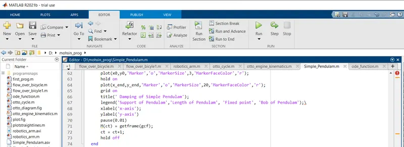
Remove the '/' operator from the code.

• The variable videofile doesn't initialise as command is incorrect.

Using of 'VideoWriter' instead of videoWriter.

RESULTS :

• A plot is drawn between angular velocity, angular displacement to the time span.

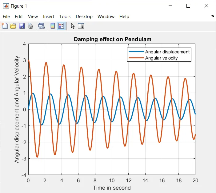
The Blue curve represents the angular displacement starts from 0 and the orange curve represents the angular velocity starts from 3 radian/second.

• The link of the animation of damping effect on simple pendulum is given below,

https://www.youtube.com/watch?v=f8ZJp4SA3X8

CONCLUSION :

• As seen in the graph, the periodic curve of Angular Displacement and Angular Velocity reduces with respect to time. This is mainly due to the damping factor. It can also be stated as the simple pendulum is subjected to a restoring force due to damping factor that will accelerate it back towards the equilibrium position. This is why the motion of simple pendulum is called as damped simple harmonic motion.
• From the animation of motion of the simple pendulum, it can be concluded that, as the damping coefficient is increased, the motion of the pendulum reduces correspondingly and approaches the equilibrium position. Also increase in damping coefficient reduces the time taken by the pendulum to reach its equilibrium position and vice-versa.