AIM

To write a code to calculate the global maxima of stalagmite function using Genetic Algorithm in MATLAB.

OBJECTIVES

The objective of the report is to optimise the stalagmite function by coding the program with the help of genetic algorithm in MATLAB  and explain the concept of genetic algorithm and also explain the syntax of ‘ga’ in MATLAB

STALAGMITE

Stalagmite is a type of rock formation that rises from the floor of a cave due to the accumulation of material deposited on the floor from ceiling drippings. Stalagmites are typically composed of calcium carbonate, but may consist of lava, mud, peat, pitch, sand, sinter and amberat (crystallized urine of pack rats).

Since our function givers a shape of stalagmite it is named as stalagmite function. Stalagmite function is a mathematical model that help us to generate minimas and maximas .it is 3D function and is designate to generate local maximas.

THEORY OF GENETIC ALGORITHM

Genetic Algorithm (GA) is a search-based optimization technique based on the principles of Genetics and Natural Selection. It is frequently used to find optimal or near-optimal solutions to difficult problems which otherwise would take a lifetime to solve. It is frequently used to solve optimization problems, in research, and in machine learning.

OPTIMISATION: Optimization is the process of making something better. In any process, we have a set of inputs and a set of outputs as shown in the following figure.

Optimization refers to finding the values of inputs in such a way that we get the “best” output values. The definition of “best” varies from problem to problem, but in mathematical terms, it refers to maximizing or minimizing one or more objective functions, by varying the input parameters.

The set of all possible solutions or values which the inputs can take make up the search space. In this search space, lies a point or a set of points which gives the optimal solution. The aim of optimization is to find that point or set of points in the search space.

A genetic algorithm is a search heuristic that is inspired by Charles Darwin’s theory of natural evolution. This algorithm reflects the process of natural selection where the fittest individuals are selected for reproduction in order to produce offspring of the next generation.

NOTION OF NATURAL SELECTION

The process of natural selection starts with the selection of fittest individuals from a population. They produce offspring which inherit the characteristics of the parents and will be added to the next generation. If parents have better fitness, their offspring will be better than parents and have a better chance at surviving. This process keeps on iterating and at the end, a generation with the fittest individuals will be found.

This notion can be applied for a search problem. We consider a set of solutions for a problem and select the set of best ones out of them.

Five phases are considered in a genetic algorithm.

1. Initial population
2. Fitness function
3. Selection
4. Crossover
5. Mutation

Initial Population

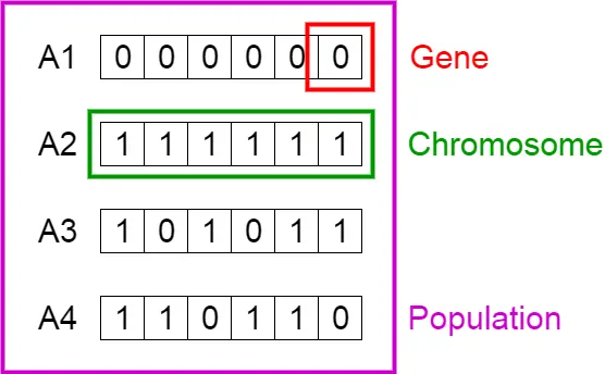
The process begins with a set of individuals which is called a Population. Each individual is a solution to the problem you want to solve.

An individual is characterized by a set of parameters (variables) known as Genes. Genes are joined into a string to form a Chromosome (solution).

In a genetic algorithm, the set of genes of an individual is represented using a string, in terms of an alphabet. Usually, binary values are used (string of 1s and 0s). We say that we encode the genes in a chromosome.

Fitness Function

The fitness function determines how fit an individual is (the ability of an individual to compete with other individuals). It gives a fitness score to each individual. The probability that an individual will be selected for reproduction is based on its fitness score.

Selection

The idea of selection phase is to select the fittest individuals and let them pass their genes to the next generation.Two pairs of individuals (parents) are selected based on their fitness scores. Individuals with high fitness have more chance to be selected for reproduction.

Crossover

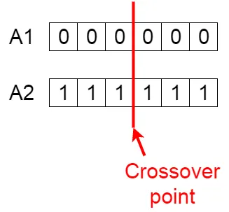
Crossover is the most significant phase in a genetic algorithm. For each pair of parents to be mated, a crossover point is chosen at random from within the genes.For example, consider the crossover point to be 3 as shown below.

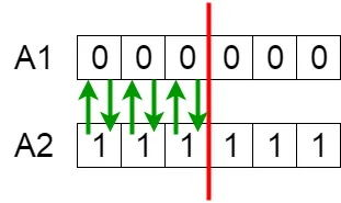
Offspring are created by exchanging the genes of parents among themselves until the crossover point is reached.\

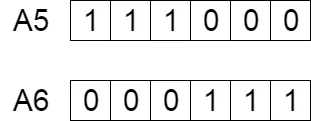
The new offspring are added to the population.

Mutation

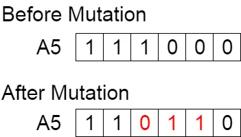
In certain new offspring formed, some of their genes can be subjected to a mutation with a low random probability. This implies that some of the bits in the bit string can be flipped.

TERMINATION

The algorithm terminates if the population has converged (does not produce offspring which are significantly different from the previous generation). Then it is said that the genetic algorithm has provided a set of solutions to our problem.

GOVERNING EQUATION 

To generate the stalagmite function the following function is used.

`f1(x) = (sin(5.1*pi*x + 0.5))^2`

`f1(y) = (sin(5.1*pi*y + 0.5))^2`

`f2(x) = exp(-4*log2*(x - 0.0667)^2)/0.64`

`f2(y) = exp(-4*log2*(y - 0.0667)^2)/0.64`

maximising f(x,y)  is the same as the mismising -f(x,y)

GENETIC ALGORITHM - SYNTAX

function  v  = stalagmite(input)
x = input(1);
y = input(2);
f1x = (sin(5.1*pi*x + 0.5))^6;
f1y = (sin(5.1*pi*y + 0.5))^6;

f2x = exp(-4*log(2)*((x - 0.0667)^2)/0.64);
f2y = exp(-4*log(2)*((y - 0.0667)^2)/0.64);

 v  = -(f1x*f1y*f2x*f2y) ;
end

EXPLANATION:

Create function program for a stalagmite function

function  v  = stalagmite(input)

give input values to stalagmite function to calculate the values in formula

x = input(1);

y = input(2);

use equation of stalagmite function in a program to find the function value.

f1x = (sin(5.1*pi*x + 0.5))^6;

f1y = (sin(5.1*pi*y + 0.5))^6;

f2x = exp(-4*log(2)*((x - 0.0667)^2)/0.64);

f2y = exp(-4*log(2)*((y - 0.0667)^2)/0.64);

  v  = -(f1x*f1y*f2x*f2y)

Finally we find the f value for the stalagmite function and end the function program.

PROGRAM

CODE FOR FINDING GLOBAL MAXIMA:

clear all
close all
clc

%defining our search space
x = linspace(0,0.6,150);
y = linspace(0,0.6,150);

%creating 2d array
[ xx yy ] = meshgrid(x,y);

%calculating fitting function
 for i = 1:length(xx)
     for j= 1:length(yy)
         input(1) = xx(i,j);
          input(2) = yy(i,j);
          f(i,j) = stalagmite(input);
     end
 end
 
 %plotting stalagmite function
 surf(xx,yy,-f)
 shading interp
 % performing the genetic algorithm
 [input fval ] = ga(@stalagmite,2)
 x_opt = input(1)
 y_opt = input(2)
 f_opt = fval
 
 

STUDY 1 : STATISTICAL BEHAVIOUR 

CODE: 

clear all
close all
clc

%defining our search space

x = linspace(0,0.6,150);
y = linspace(0,0.6,150);
%creating 2d array
[ xx yy ] = meshgrid(x,y);
 for i = 1:length(xx)
     for j= 1:length(yy)
         input(1) = xx(i,j);
          input(2) = yy(i,j);
          f(i,j) = stalagmite(input);
     end
 end
 num_cases = 50;
 tic
 % study1  - Statistical study_ performing the genetic algorihtm
for i =1:num_cases
    [ inputs1,fopt1(i) ] = ga(@stalagmite,2);
    xopt1(i) = inputs1(1);
    yopt1(i) = inputs1(2);
end
%global maxima and function values
study_time = toc
figure(1)
subplot(2,1,1)
hold on
surfc(xx,yy,-f)
shading interp
plot3(xopt1,yopt1,-fopt1,'marker','o','markersize',5,'markerfacecolor','r')
xlabel('x-value')
ylabel('y-value')
title('unbounded plot')
subplot(2,1,2)
plot(-fopt1)
xlabel('Iterations')
ylabel('Function maxima')
title('variation in F')

STUDY 2 : STATISTICAL BEHAVIOUR  - WITH BOUNDED UNPUTS

clear all
close all
clc
%defining our search space

x = linspace(0,0.6,150);
y = linspace(0,0.6,150);
%creating 2d array
[ xx yy ] = meshgrid(x,y);
 for i = 1:length(xx)
     for j= 1:length(yy)
         input(1) = xx(i,j);
          input(2) = yy(i,j);
          f(i,j) = stalagmite(input);
     end
 end
 num_cases = 50;
options = optimoptions('ga')
 options = optimoptions(options,'populationsize',170);
  
 % study 2 - Statistical study - with upper and lower bounds
  tic
  % performing genetic algorithm
for i =1:num_cases
    [ inputs2,fopt2(i) ] = ga(@stalagmite,2,[],[],[],[],[0;0],[1;1]);
    xopt2(i) = inputs2(1);
    yopt2(i) = inputs2(2);
end
study_time = toc

% Plotting global maxima and function values
figure(2)
subplot(2,1,1)
hold on
surfc(xx,yy,-f)
shading interp
plot3(xopt2,yopt2,-fopt2,'marker','o','markersize',5,'markerfacecolor','r')
xlabel('x-value')
ylabel('y-value')
title('bounded plot')
subplot(2,1,2)
plot(-fopt2)
xlabel('Iterations')
ylabel('Function maxima')
title('variation in F')

STUDY 3 - STATISTICAL BEHAVIOUR WITH BOUNDED INPUTS AND INCREASED POPULATION

CODE:

clear all
close all
clc
%defining our search space

x = linspace(0,0.6,150);
y = linspace(0,0.6,150);
%creating 2d array
[ xx yy ] = meshgrid(x,y);
 for i = 1:length(xx)
     for j= 1:length(yy)
         input(1) = xx(i,j);
          input(2) = yy(i,j);
          f(i,j) = stalagmite(input);
     end
 end
 num_cases = 50;

 % study 3 - Increasing GA iteration
 options = optimoptions('ga')
 options = optimoptions(options,'PopulationSize',300);
 tic
 % performing genetic algorithm
for i =1:num_cases
    [ inputs3,fopt3(i) ] = ga(@stalagmite,2,[],[],[],[],[0;0],[0.2;0.2],[],[],options);
    xopt3(i) = inputs3(1);
    yopt3(i) = inputs3(2);
end
study3_time = toc

%plotting global maxima and function values
figure(3)
subplot(2,1,1)
hold on
surfc(xx,yy,-f)
shading interp
plot3(xopt3,yopt3,-fopt3,'marker','o','markersize',5,'markerfacecolor','r')
xlabel('x-value')
ylabel('y-value')
title('bounded input and increasing ')
subplot(2,1,2)
plot(-fopt3)
xlabel('Iterations')
ylabel('Function maxima')
title('Variation in F')
fprintf('the function value')
disp(-fopt3(num_cases))

EXPLANATION FOR CALCULATING A GLOBAL MAXIMA PROGRAM

1. Give the range of x and y value in ‘linspace’ command to get a value in matrix.
2. Use the ‘meshgrid’ command to get a matrix vaoue of xx and yy.
3. Use ‘for’ loop to finding the stalagmite function value for x and y values.
4. In for loop to calling the ‘ stalagmite function program’ for finding the f values (use -ve sign to find the global maxima)
5. After finding the function value (f value) use surf to plot the values.
6. Using ‘shade interp ' to hide the lines in the stalagmite plot.
7. Use ‘ga' to find the global maxima and minima l, local maxima and minima in the stalagmite function. In MATLAB ga will give only minima value.
8. Give ‘num_cases’ value to run the number of ga iteration.
9. In study 1 – Statistical Behaviour webget ‘unbounded inputs ‘ using the ga syntax of x= ga ( fun, nvars); and finding the xopt, yopt, values using for loop.
10. Use ‘subplot’ to get two plots in a single figure.
11. Use ‘plot3’ command to plot three values in a single plot.
12. Use onother ‘subplot’ to get another plot in a above figure (1) window.
13. Use 'plot' command to plot the (-fopt) value in figure (1) window.
14. Use 'xlabel' 'ylabel' to command the name of xvalues and y values.
15. Use 'tic' and 'toc' command to calaculate the time of getting output for study 1.
16. In study 2- statistical behavior with upper and lower bounds we get the ‘bounded inputs’ and finding the xopt, yopt values using ‘for loop’.
17. Use 'subplot' 'plot3' 'plot' 'xlabel' 'ylabel' 'tic' and 'toc' command similary to study 1.
18. In study 3 -Increasing GA iterations we get the ‘Global maxima’ using the ga syntax of x.
19. Use 'subplot' 'plot3' 'plot' 'xlabel' 'ylabel' 'tic' and 'toc' command similary to study 1 And study 2.
20. Use fprintf command to get the function value and the function value must be in postive because we are finding the global maxima values.
21. Finally prews the run button to run the program and getting the output of global maxima.

OUTPUT FOR CALCULATION A GLOBAL MAXIMA OF A STALAGMITE FUNCTION USING GENETIC ALGORITHM

FIGURE 1 : CONSIDERING INPUT RANGE

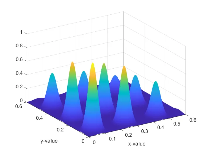
FIGURE 2: STUDY 1 - STATISTICAL BEHAVIOUR

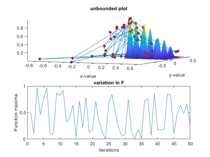
study_time =    2.9995

In this study we do the genetic algorithm without setting any bounds and hence we get result for x and y outside the domain as well as many values ,because of which single value cannot be determined 

FIGURE 3: STUDY 2- STATISTICAL BEHAVIOUR- with upper bounds and lower bounds 

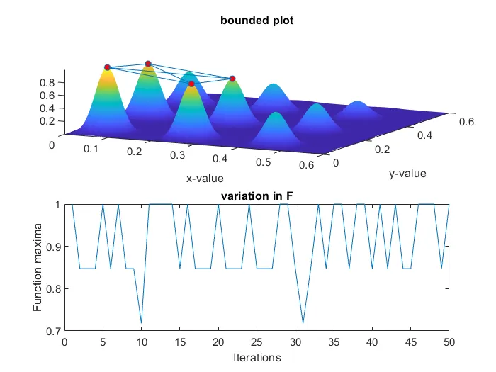
study_time = 3.4500

In this study ,we set the bounds of x and y as shown in the code and the syntax . as we set the bounds, the most likely answer is coming near 3 peak as shown in the figure and the minimum value ranges between 0 and 1 . To get more refined we will increase the population size in the next study.

FIGURE 4: STUDY 2-INCREASING GA ITERATION BY GIVING POPULATION SIZE 

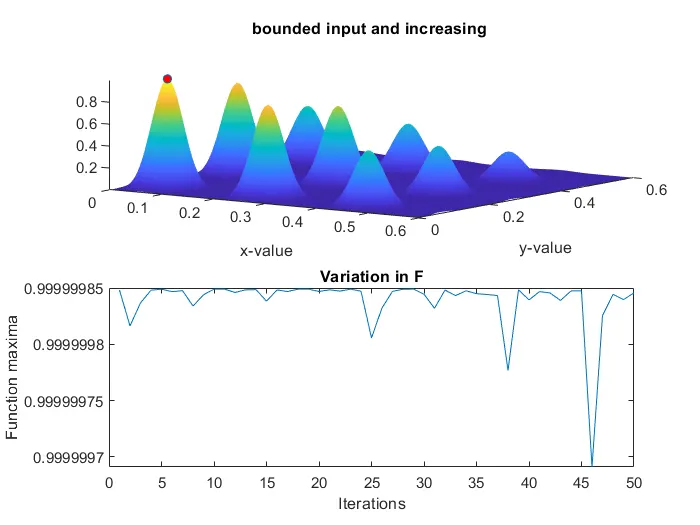
study_time =  11.1659

To get proper and considerable result we will increase the population size of GA using optimoptions so that more generations and off springs are produced that will lead the result towards convergence.

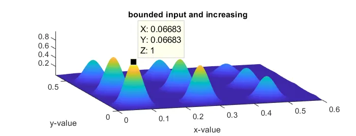
 Here we increase the population size to 300 so that we get a optimised value . Now we only see only one red dot which is the maximum value of the function which comes out to be 1 .

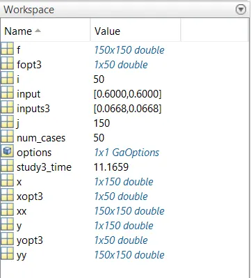
The optimum value of   [ xopt  yopt ] =  [ 0.06683 0.06683 ] ,   which is shown below

WORKSPACE 

CONCLUSION

Hence we are able to optimise the stalagmite function and find the global maxima of the function.

The GA is only used for the minimum function therefore to maximize the function we inversed the  minimum function.

INFERENCE

https://www.tutorialspoint.com/genetic_algorithms/genetic_algorithms_introduction.htm

https://en.wikipedia.org/wiki/Genetic_algorithm

https://in.mathworks.com/help/gads/ga.html#d120e39545