Week 3 - Solving second order ODEs

AIM

To solve a matlab program to simulate the motion of a simple pendulum with damping.

GOVERNING EQUATIONS

When a simple pendulum is swung it eventually comes to rest because of gravity and air friction so the equation of motion for a pendulum with damping which follows a second order ODE is as follows:

`d^2 θ/dt^2 + (b/m)*dθ/dt + (g/L)*sinθ =0`

Where,

`θ` = angular displacement of the pendulum

t= time

b = damping coefficient

m = mass of the bob

g = gravity

L = length of the pendulum

Solving the above equation tracks the motion of the pendulum with considering the effect of air friction and gravity.

In Matlab,second order differential eqns are not solved but they can be converted in to 2 first order differential equation , then we can use the ode45 function. The syntax for ode45 is [t,y] = ode45@(t,y),odefun,tspan,y0,options) so convert the above eqn in 2 first order eqns it is done as follows

`d/dt[ θ2] = -(b/m)* θ2– (g/l)*sin(θ1)`

now we can program the pendulum motion in matlab

dθ/dt = angular velocity = `θ1

`d^2 θ/dt^2` = angular acceleration = θ2

PROCEDURE

• Lower the order of ODE using substitution method.Prepare a function for the same for code neatness purpose.
• Set the geometrical and physical parameters of the pendulum like length,mass,damping coefficient as well as gravity.
• Set the initial condition and timespan for which you want to run the simulation.
• Use the inbuilt ODE solver named ODE45 to solve ODE which is reduced by calling our function that is made un step1 and obtain values of displacement and velocity and store it in a array.
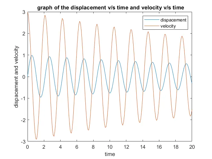
• Plot the graph of the displacement v/s time and velocity v/s time
• Create simulation of the positions of the pendulum bob and arm using movie function.

MATLAB CODE

CODE FOR THE FUNCTION OF ODE REDUCTION:

function [ dtheta_dt ] = ode_func(t,theta,m,l,g,b)

theta1 = theta(1);
theta2 = theta(2);
dtheta1_dt = theta2;

dtheta2_dt = -(b/m)*theta2 - (g/l)*sin(theta1);
dtheta_dt = [ dtheta1_dt;dtheta2_dt ];

end

Code explanation

• Refer the governing equation section. The steps followed in that section have been converted in to matlab code likewise.
• The only addition is that the final derivation of theta1 and theta2 is stored in an array because of presence of multiple values.

Code for main program

close all
clear all
clc
% given conditions
b = 0.05;
m =1;
l = 1;
g = 9.81;

% initial condition 
theta_0 = [0;3];
% time points 
t_span = linspace(0,20,200);
% solve ode

[t,results] = ode45(@(t,theta) ode_func(t,theta,m,l,g,b),t_span,theta_0);

% Plot the graph of the displacement v/s time and velocity v/s time
figure(1)
plot(t,results)
legend('dispacement_time ','velocity_time')
xlabel('time')
ylabel('dispacement and velocity')
title(' graph of the displacement v/s time and velocity v/s time')

ct = 1;
for i = 1:length(results(:,1))
    % set the hinge points
 x0 = 0;
y0 = 0; 
% getting coordinates from trignometry
 x1 = l*sin(results(i,1));
 y1 = -l*cos(results(i,1));
% plotting lines from hinge to the end witha ball marker at the end
figure(2)
plot([x0 x1],[y0 y1],'linewidth',2)
hold on
plot(x1,y1,'marker','o','markerfacecolor','b','markeredgecolor','r','markersize',20)
hold off
axis([-1 1 -1.5 0])
pause(0.01)
  M(ct) = getframe(gcf);
  

ct= ct + 1;

end
% joining each frame and making a movie
movie(M);
%creating a video file
videofile = VideoWriter('ODE_solution.avi','uncompressed AVI')
open(videofile)
% writing the data to a video file
writeVideo(videofile,M)
close(videofile)

CODE EXPLANATION

• Set physical parameters of the pendulum like mass, length ,gravity and damping coefficient.
• Set the initial conditions and timespan for which you want to run the simulation
• T0 use ode solver ,use ode45 function which main inputs as (t,theta) while you use ode_func with inputs as (t,theta,l,b,g,m) and t_span and theta_0 as the initial condition.
• These results are stored in an array of [t,results]
• Since results contain 2 components, angular displacemet and velocity ,to plot both the graphs ,use the (:,1) and (:,2) and plot the graph.
• To create animation use ‘for’ loop so that we can get the x and y coordinates
• Use the pause() function to give a pause for evey looping of values.
• Use movie making command as per code to create an animation.

OBSERVATION

Graph of the displacement v/s time and velocity v/s time

GOOGLE DRIVE LINK TO SHOW THE ANIMATION OF A SIMPLE PENDULUM IN MATLAB:

https://drive.google.com/file/d/1f_Xrn76piOrzG27nLB20kPP27r5-beHI/view?usp=sharing

CONCLUSION

The reduction in angle displacement and velocity is due to damping is due to the damping coefficient indroduced in the second order ODE of a simple pendulum.

We have successfully solved the second order ODE.

The animation of the pendulum is shown.