Project 2 - Rankine cycle Simulator
AIM:
The Rankine cycle is the fundamental operating cycle of all power plants where an operating fluid is continuously evaporated and condensed. Inthis mechanism, fuel is used to produce heat within a boiler, converting water into steam which then expands through a turbine producing usefulwork. In this project, we are going to create a Rankine Cycle Simulator using MATLAB. This Simulator can be used to calculate the useful data from a set of inputs of the cycle & also plot the thermodynamic properties. This simulator can be used as a tool that predicts the performance of the cycleunder given conditions.
THEORY
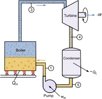
The Rankine cycle is the fundamental operating cycle of all power plants where an operating fluid is continuously evaporated and condensed. The selection of operating fluid depends mainly on the available temperature range. Figure 1 shows the idealized Rankine cycle.
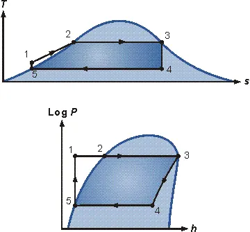
The pressure-enthalpy (p-h) and temperature-entropy (T-s) diagrams of this cycle are given in Figure 2. The Rankine cycle operates in the following steps:
-
1-2-3 Isobaric Heat Transfer. High pressure liquid enters the boiler from the feed pump (1) and is heated to the saturation temperature (2). Further addition of energy causes evaporation of the liquid until it is fully converted to saturated steam (3).
-
3-4 Isentropic Expansion. The vapor is expanded in the turbine, thus producing work which may be converted to electricity. In practice, the expansion is limited by the temperature of the cooling medium and by the erosion of the turbine blades by liquid entrainment in the vapor stream as the process moves further into the two-phase region. Exit vapor qualities should be greater than 90%.
-
4-5 Isobaric Heat Rejection. The vapor-liquid mixture leaving the turbine (4) is condensed at low pressure, usually in a surface condenser using cooling water. In well designed and maintained condensers, the pressure of the vapor is well below atmospheric pressure, approaching the saturation pressure of the operating fluid at the cooling water temperature.
-
5-1 Isentropic Compression. The pressure of the condensate is raised in the feed pump. Because of the low specific volume of liquids, the pump work is relatively small and often neglected in thermodynamic calculations.
- figure 1
- figure 2
GOVERNING EQUATIONS
Work is done at the pump will be calculated as.
`Wp = h4 – h3`
Work is done at the Turbine will be calculated as.
`Wr=hl – h2`
The Net-work done will be calculated as.
`Wnt = Wp - WT`
The efficiency of the cycle will be calculated.
`n = (WT-Wp)/(Qi) * 100`
The heat input.
`Qi= hl – h4`
The heat output.
`Qout = h2 - h3`
Back work ratio.
`BWR = (Wp)/(Wt)`
Specific steam consumption of the turbine.
`SSC = (Wnt)/3600`
Where,
h1, h2, h3, h4 are the enthalpies at state points 1, 2, 3, 4 respectively.
MATLAB CODE :
clear all
close all
clc

disp('Rankine Cycle Simulator')
disp('process 1-2: Isentropic expansion in turbine ')
disp('process 2-3: constant pressure heat rejection in condenser')
disp('process 3-4: Isentropic Compression in pump')
disp('process 4-1: constant pressure heat addition in boiler')

% Intial data inputs
T1 = input('Enter the turbine inlet temp: ');
p1 = input('Enter the turbine inlet press: ');
p2 = input('Enter the Condensor inlet press: ');


% State Point 1 parameters i.e Turbine Inlet
Tsat = XSteam('Tsat_p',p1);

h1 = XSteam('h_pt',p1,T1);
s1 = XSteam('s_pt',p1,T1);

%State Point 2 parameters i.e Condenser Inlet
s2 = s1;
sf2 = XSteam('sL_p',p2);
sg2 = XSteam('sv_p',p2);

% s2=sf2+(x2*sfg2)
% Dryness fraction
x2 =(s2-sf2)/(sg2-sf2);

T2 = XSteam('T_ps',p2,s2);
h2 = XSteam('h_px',p2,x2);
hf2 = XSteam('hL_p',p2);

% State Point 3 Parameters i.e Pump Inlet
p3 = p2;
T3 = T2;
s3 = sf2;
h3 = hf2;
T5 = Tsat;

% State Point 4 Parameters i.e Boiler Inlet
s4 = s3;
p4 = p1;
h4=XSteam('h_ps',p4,s4);
cp=XSteam('cp_ps',p4,s4);
cv=XSteam('cv_ps',p4,s4);
c=cp/cv;
T4=T3*((p4/p3)^(c-1)/c)

% State Point 5,6 Parameters
T5=Tsat;
h5=XSteam('hL_p',p1);
s5=XSteam('sL_p',p1);
T6=T1;
h6=XSteam('hV_p',p1);
s6=XSteam('sV_p',p1);

% Plotting T-S Diagram (saturation line curve)
t=linspace(5,400,25000);
for i=1:length(t)
s(i)=XSteam('sL_t',t(i));
S(i)=XSteam('SV_t',t(i));
h(i)=XSteam('hL_t',t(i));
H(i)=XSteam('hV_t',t(i));
end
figure(1)
plot(s,t,'linewidth',2);
hold on
plot(S,t,'linewidth',2);

plot([s1,s2,s3,s4,s5,s6],[T1,T2,T3,T4,T5,Tsat],'linewidth',2,'color','k');
text(s1+0.1, T1, '1')
text(s2+0.1, T2, '2')
text(s3, T3-20, '3')
text(s4, T4+20, '4')
axis([-3,10,10,500]);


% Plotting Saturated Temperature
a=linspace(Tsat,T1,500);
for i=1:length(a)
    m(i)=XSteam('s_pt',p1,a(i));
end
plot(m,a,'linewidth',2,'color','k')
title('Temperature vs Entropy')
xlabel('Entropy(S)- kJ/kg K')
ylabel('Temperature(T)-degree C')
legend('Liquid Phase','Vapour Phase')

%plotting S H diagram

figure(2)
plot(s,h);
hold on
plot(S,H);

plot([s1,s2,s3,s4,s5,s6,s1],[h1,h2,h3,h4,h5,h6,h1],'linewidth',2,'color','k');
text(s1+0.1, h1, '1')
text(s2+0.1, h2, '2')
text(s3, h3-100, '3')
text(s4, h4 +200, '4')
title('Enthalpy vs Entropy')
xlabel('Entropy(S)- kJ/kg K')
ylabel('Enthalpy(h)-kJ/kg')
legend('Liquid Phase','Vapour Phase','location','northwest')

% Result to be displayed in the command window
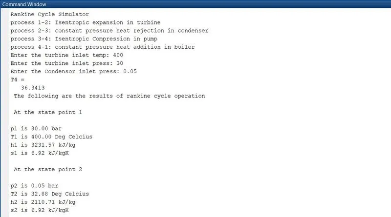
disp(' The following are the results of rankine cycle operation ')
disp(' ')
disp(' At the state point 1')
disp(' ')
n1=sprintf('p1 is %.2f bar',p1);
disp(n1)
n2=sprintf('T1 is %.2f Deg Celcius',T1);
disp(n2)
n3=sprintf('h1 is %.2f kJ/kg',h1);
disp(n3)
n4=sprintf('s1 is %.2f kJ/kgK',s1);
disp(n4)

disp(' ')
disp(' At the state point 2')
disp(' ')
n5=sprintf('p2 is %.2f bar',p2);
disp(n5)
n6=sprintf('T2 is %.2f Deg Celcius',T2);
disp(n6)
n7=sprintf('h2 is %.2f kJ/kg',h2);
disp(n7)
n8=sprintf('s2 is %.2f kJ/kgK',s2);
disp(n8)

disp(' ')
disp(' At the state point 3')
disp(' ')
n9=sprintf('p3 is %.2f bar',p3);
disp(n9)
n10=sprintf('T3 is %.2f Deg Celcius',T3);
disp(n10)
n11=sprintf('h3 is %.2f kJ/kg',h3);
disp(n11)
n12=sprintf('s3 is %.2f kJ/kgK',s3);
disp(n12)

disp(' ')
disp(' At the state point 4')
disp(' ')
n13=sprintf('p4 is %.2f bar',p4);
disp(n13)
n14=sprintf('T4 is %.2f Deg Celcius',T4);
disp(n14)
n15=sprintf('h4 is %.2f kJ/kg',h4);
disp(n15)
n16=sprintf('s4 is %.2f kJ/kgK',s4);
disp(n16)


% Workdone by turbine

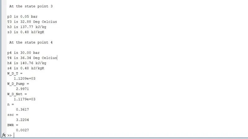
W_D_T = h1-h2

% Workdone by the pump

W_D_Pump = h4-h3

%net workdone

W_D_Net = W_D_T-W_D_Pump

% Heat Supplied
q = h1-h4;

% Effeciency
n = W_D_Net/q

% Specific steam consumption
ssc = 3600/W_D_Net

% Back Work Ratio
BWR = W_D_Pump/W_D_T
CODE EXPLANATION
We start the code with regular usual commands by using clear all ; close all; clc; for clearing the windows with previous data and closing any previous figures/plots generated.
- Ist various processes from 1-4 for Rankine cycle are printed using fprintf command.
- Initializing the known variables by giving the input using input command for T1, P1 & P2 variables.
- Then extracting all the required values from the XSteam.m file library which act as a Standard Steam table to calculate the values for state points.
- By using XSteam library file we call it by XSteam in MATLAB then required function are taken and then giving the input accordingly to that particular function like in case of State point 1 input given is P1 & T1.
- Similarly, state point 2,3, & 4 are calculated for Enthalpy, Entropy, Pressure & Temperature using XSteam functions.
- Next calculation had been done by using the basic formulae for Work done (W.D) and Heat transferred (Q) in the Rankine cycle along with the thermal efficiency respectively.
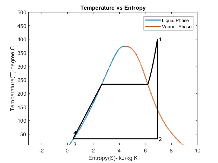
- Then, temperature range has been specified using linspace command & figure 1 has been plotted in which the for loop is used logically to construct the saturation curve in graph.
- Finally, for figure 1 Temperature vs Entropy has been plotted using plot command by mentioning S1 to S6 for X-axis & T1 to Tsat points for Y- axis along with plotting for saturated cuvre respectively.
- A command named text is used further in last step for plotting the T-S graph in which text command is used add text descriptions to data points like 1,2,3 & 4 we had added easily. Syntax used for text command - text(x,y,text)
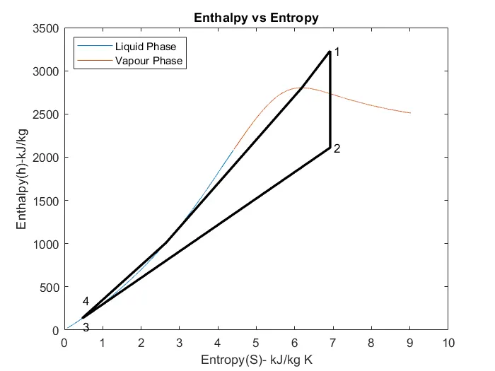
- Same procedure which is used to plot T-S graph had been followed and coded further for H-S Enthalpy vs Entropy Graph to get the output.
In the final step all the calculated state points and the necessary values like net work done, efficiency, back ratio, etc had been printed step by step using fprintf command in MATLAB respectively.
RESULTS
T S DIAGRAM
H S DIAGRAM
COMMAND WINDOW
CONCLUSION
- Rankine cycle is use in Thermal power plant so it is vital to understand as its help to calculate all the properties of the steam so that it gives ease to improve power output and efficiency of the plant.
- As water is the working fluid it is necessity to understand all its properties for this cycle, which we get to learn in this project.
- Setting/coding one program to calculate all the plots/figures and steam property at every stage of Rankin cycle will we easy for any one, as one have to put just three input, p1, T1 and p2, even non-technical person can simulate it.
- At last, This simulator help to reduce enormous amount of time to generate results.
REFERENCE
https://www.thermopedia.com/content/1072/