Week 4.1 - Genetic Algorithm

A genetic algorithm (GA) is a search-based optimization technique based on the principles of Genetics and Natural Selection. It is frequently used to find optimal or near-optimal solutions to difficult problems which otherwise would take a lifetime to solve.

Advantages of GAs

GAs have various advantages which have made them immensely popular. These include −

• Does not require any derivative information (which may not be available for many real-world problems).
• Is faster and more efficient as compared to the traditional methods.
• Has very good parallel capabilities.
• Optimizes both continuous and discrete functions and also multi-objective problems.
• Provides a list of “good” solutions and not just a single solution.
• Always gets an answer to the problem, which gets better over time.

Useful when the search space is very large and there are a large number of parameters involved.

Basic Structure

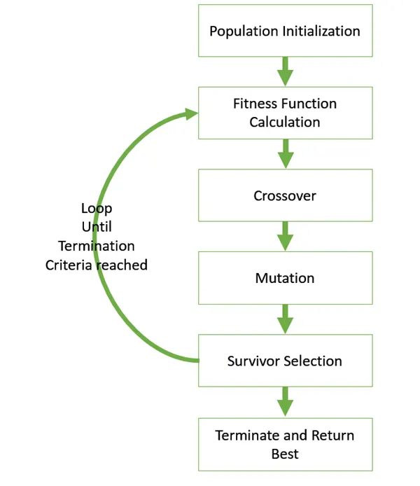
The basic structure of a GA is as follows −

We start with an initial population (which may be generated at random or seeded by other heuristics), select parents from this population for mating. Apply crossover and mutation operators on the parents to generate new off-springs. And finally, these off-springs replace the existing individuals in the population and the process repeats. In this way, genetic algorithms actually try to mimic human evolution to some extent.

Each of the following steps is covered as a separate chapter later in this tutorial.

Basic Terminology

Before beginning a discussion on Genetic Algorithms, it is essential to be familiar with some basic terminology that will be used throughout this tutorial.

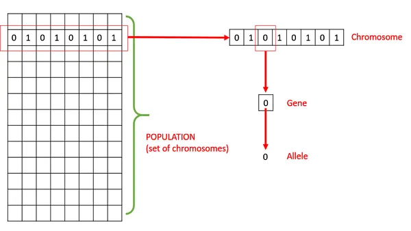
• Population− It is a subset of all the possible (encoded) solutions to the given problem. The population for a GA is analogous to the population for human beings except that instead of human beings, we have Candidate Solutions representing human beings.
• Chromosomes− A chromosome is one such solution to the given problem.
• Gene− A gene is one element position of a chromosome.
• Allele − It is the value a gene takes for a particular chromosome.

• Genotype− Genotype is the population in the computation space. In the computation space, the solutions are represented in a way that can be easily understood and manipulated using a computing system.
• Phenotype− Phenotype is the population in the actual real-world solution space in which solutions are represented in a way they are represented in real-world situations.
• Decoding and Encoding− For simple problems, the phenotype and genotype spaces are the same. However, in most of cases, the phenotype and genotype spaces are different. Decoding is a process of transforming a solution from the genotype to the phenotype space, while encoding is a process of transforming from the phenotype to the genotype space. Decoding should be fast as it is carried out repeatedly in a GA during the fitness value calculation.

%program to optimise the stalagmite function and find the global maxima of the function.

%program to optimize the stalagmite function and find the global maxima of the function.

clear all
close all
clc

%defining search space
x = linspace(0,0.6,150);
y = linspace(0,0.6,150);
num_cases = 50;

%creating a 2d mesh
[xx,yy] = meshgrid(x,y);

%Evaluating the stalagmite function
for i = 1:length(xx)
    for j = 1:length(yy)
        input_vector(1)=xx(i,j);
        input_vector(2)=yy(i,j);
        f(i,j) = get_stalagmite(input_vector);
    end
end

tic
% study 1 - statistical behaviour
for i = 1:num_cases
    [inputs,fopt1(i)] = ga(@get_stalagmite,2);
    xopt1(i) = inputs(1);
    yopt1(i) = inputs(2);
end
study1_time = toc

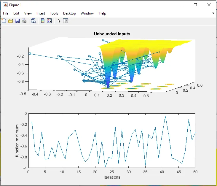
figure(1)
subplot(2,1,1)
hold on
surfc(x,y,f)
shading interp
plot3(xopt1,yopt1,fopt1,'marker','o','markersize',5)
title('Unbounded inputs')
subplot(2,1,2)
plot(fopt1)
xlabel('iterations')
ylabel('function minimum')

tic
%study 2 - statistical behaviour-with upper and lower bounds
for i = 1:num_cases
    [inputs,fopt2(i)] = ga(@get_stalagmite,2,[],[],[],[],[0;0],[0.6,0.6]);
    xopt2(i) = inputs(1);
    yopt2(i) = inputs(2);
end

study2_time = toc

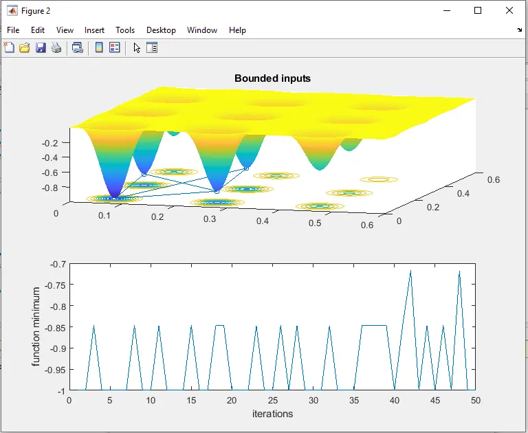
figure(2)
subplot(2,1,1)
hold on
surfc(x,y,f)
shading interp
plot3(xopt2,yopt2,fopt2,'marker','o','markersize',5)
title('Bounded inputs')
subplot(2,1,2)
plot(fopt2)
xlabel('iterations')
ylabel('function minimum')


%study 3 - Increasing GA Iterations
options = optimoptions('ga');
options = optimoptions(options,'PopulationSize',170);


tic
for i = 1:num_cases
    [inputs,fopt3(i)] = ga(@get_stalagmite,2,[],[],[],[],[0;0],[0.6;0.6],[],[],options)
     xopt3(i) = inputs(1);
     yopt3(i) = inputs(2);
end
study3_time=toc
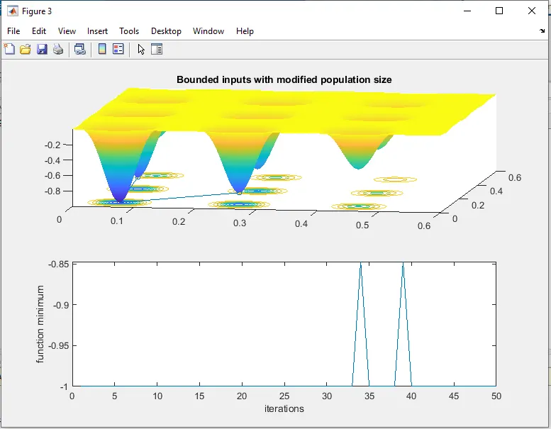
figure(3)
subplot(2,1,1)
hold on
surfc(x,y,f)
shading interp
plot3(xopt3,yopt3,fopt3,'marker','o','markersize',5)
title('Bounded inputs with modified population size')
subplot(2,1,2)
plot(fopt3)
xlabel('iterations')
ylabel('function minimum')

%get stalagmite function
function f =get_stalagmite(input_vector)
x=input_vector(1);
y=input_vector(2);
a = [sin(5.1*pi*x+0.5)]^6;
b = [sin(5.1*pi*y+0.5)]^6;
c = exp(-4*log(2)*(x-0.0667)^2/(0.64));
d = exp(-4*log(2)*(y-0.0667)^2/(0.64));

f = -(a*b*c*d);

end

Source - Genetic Algorithms - Introduction (tutorialspoint.com)