Week 4.1 - Genetic Algorithm

AIM :

To find the global maxima of stalagmite function by optimization method using genetic algorithm.

• Write a code in MATLAB to optimise the stalagmite function and find the global maxima of the function.
• Clearly expalin the concept of genetic algorithm in your own words and also explain the syntax for ga in MATLAB in your report.
• Make sure that your code gives the same output, even if it is made to run several times.
• Plot graphs for all 3 studies and for F maximum vs no. of iterations. Title and axes labels are a must, legends could be shown if necessary.

THEORY :

The genetic algorithm is a random-based classical evolutionary algorithm. By random here we mean that in order to find a solution using the GA, random changes applied to the current solutions to generate new ones. Note that GA may be called Simple GA (SGA) due to its simplicity compared to other EAs.

GA is based on Darwin’s theory of evolution. It is a slow gradual process that works by making changes to the making slight and slow changes. Also, GA makes slight changes to its solutions slowly until getting the best solution.

Here is the description of how the GA works:

GA works on a population consisting of some solutions where the population size (popsize) is the number of solutions. Each solution is called individual. Each individual solution has a chromosome. The chromosome is represented as a set of parameters (features) that defines the individual. Each chromosome has a set of genes. Each gene is represented by somehow such as being represented as a string of 0s and 1s as in the next diagram.

Also, each individual has a fitness value. To select the best individuals, a fitness function is used. The result of the fitness function is the fitness value representing the quality of the solution. The higher the fitness value the higher the quality the solution. Selection of the best individuals based on their quality is applied to generate what is called a mating pool where the higher quality individual has higher probability of being selected in the mating pool.

The individuals in the mating pool are called parents. Every two parents selected from the mating pool will generate two offspring (children). By just mating high-quality individuals, it is expected to get a better quality offspring than its parents. This will kill the bad individuals from generating more bad individuals. By keeping selecting and mating high-quality individuals, there will be higher chances to just keep good properties of the individuals and leave out bad ones. Finally, this will end up with the desired optimal or acceptable solution.

But the offspring currently generated using the selected parents just have the characteristics of its parents and no more without changes. There is no new added to it and thus the same drawbacks in its parents will actually exist in the new offspring. To overcome such problem, some changes will be applied to each offspring to create new individuals. The set of all newly generated individuals will be the new population that replaces the previously used old population. Each population created is called a generation. The process of replacing the old population by the new one is called replacement. The following diagram summarizes the steps of GA.

There are two questions to be answered to get the full idea about GA:

1. How the two offspring are generated from the two parents?

2. How each offspring gets slightly changed to be an individual?

We will answer these questions later.

Chromosome Representation and Evaluation

There are different representations available for the chromosome and the selection of the proper representation is problem specific. The good representation is what makes the search space smaller and thus easier search.

The representations available for the chromosome including:

· Binary: Each chromosome is represented as a string of zeros and ones.

· Permutation: Useful for ordering problems such as travelling salesman problem.

· Value: The actual value is encoded as it is.

For example, if we are to encode the number 7 in binary, it might look as follows:

Each part of the above chromosome is called gene. Each gene has two properties. The first one is its value (allele) and the second one is the location (locus) within the chromosome which is the number above its value.

Each chromosome has two representations.

1. genotype: The set of genes representing the chromosome.

2. phenotype: The actual physical representation of the chromosome.

In the above example, binary of 0111 is the genotype and 7 is the phenotype representation.

After representing each chromosome the right way to serve to search the space, next is to calculate the fitness value of each individual. Assume that the fitness function used in our example is:

f(x) = 2x+2 Where x is the chromosome value

Then the fitness value of the previous chromosome is:

f(7) = 2(7)+2=16

The process of calculating the fitness value of a chromosome is called evaluation.

Initialization

After getting how to represent each individual, next is to initialize the population by selecting the proper number of individuals within it.

Selection

Next is to select a number of individuals from the population in the mating pool. Based on the previously calculated fitness value, the best individuals based on a threshold are selected. After that step, we will end selecting a subset of the population in the mating pool.

Variation Operators

Based on the selected individuals in the mating pool, parents are selected for mating. The selection of each two parents may be by selecting parents sequentially (1-2, 3-4, and so on). Another way is random selection of the parents.

For every two parents selected, there are a number of variation operators to get applied such as:

1. Crossover (recombination)

2. Mutation

The next diagram gives an example for these operators.

Crossover

Crossover in GA generates new generation the same as natural mutation. By mutating the old generation parents, the new generation offspring comes by carrying genes from both parents. The amount of genes carried from each parent is random. Remember that GA is random-based EA. Sometimes the offspring takes half of its genes from one parent and the other half from the other parent and sometimes such percent changes. For every two parents, crossover takes place by selecting a random point in the chromosome and exchanging genes before and after such point from its parents. The resulting chromosomes are offspring. Thus operator is called single-point crossover.

Note that crossover is important and without it, the offspring will be identical to its parent.

Mutation

Next variation operator is mutation. For each offspring, select some genes and change its value. Mutation varies based on the chromosome representation but it is up to you to decide how to apply mutation. If the encoding is binary (i.e. the value space of each gene have just two values 0 and 1), then flip the bit value of one or more genes.

But if the gene value comes from a space of more than two values such as 1,2,3,4, and 5, then the binary mutation will not be applicable and we should find another way. One way is by selecting a random value from such set of values as in the next diagram.

Note that without mutation the offspring will have all of its properties from its parents. To add new features to such offspring, mutation took place. But because mutation occurs randomly, it is not recommended to increase the number of genes to be applied to mutation.The individual after mutation is called mutant.

PROGRAM :

We are now evaluating the result of the function 'stalagmite' in all its iterations possible. It is running all the possible X and Y, as a double loop, and storing the results in the variable 'F'. This variable is a large array compromising all the results, 150 x 150 times.

Defining Search space & evaluating the stalagmite function :

clear all 
close all 
clc 

%Preparing the data

%defining our search space
x = linspace(0,0.6,150);
y = linspace(0,0.6,150);

% number of times genetic algorithm going to run
case_num = 50;


%Creating a 2 dimension mesh
[xx,yy]= meshgrid(x,y);

%evaluating the stalagmite function
for i = 1:length(xx);
    for j = 1:length(yy);
        input_vector(1)=xx(i,j);
        input_vector(2)=yy(i,j);
        f(i,j) = stalagmite(input_vector);
    end
end

% plotting the graphic area
figure(1)
surfc(xx,yy,-f)
%axis identification
xlabel('X value')
ylabel('Y value')
zlabel('Z value')
title('GLOBAL MAXIMA');
legend('STALAGMITE','GLOBAL MAXIMA')
%removing the 3D grid lines
shading interp
colorbar

After, we are plotting this first results on a 3D plot. The command 'surfc' is use to define the area of the plot, as a surface. We are using the values in the vector, xx and yy and for the third dimension, the third axis z, the value of the funtion is used.

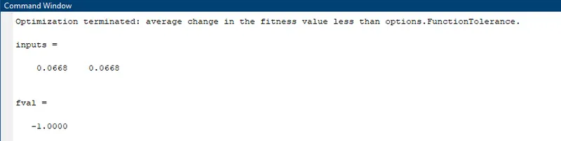
As a final step, we are applying the genetic algorithm to attemp to get the minimal value of the function. Because there is no optimization, we don't consistently get the same results. We have a good estimate, of the x and y values that are giving us that aproximation. We can see it on the 3D plot.

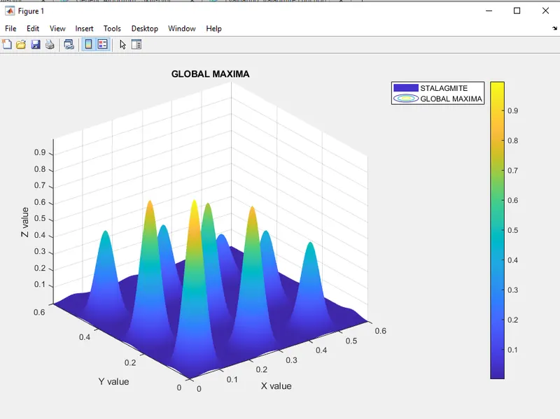
stalagmite function :

The relation of stalagmite function for global minima is given as;

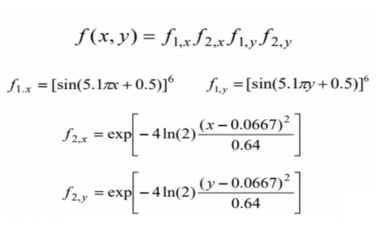
Fig: Equation of stalagmite function for Global Minima

From the above equations, we can create the function of stalagmite.

But, with the above mentioned formula, we can find the global minima. To find global maxima there is a small spin to it.

function [f] = stalagmite(input_vector)

x= input_vector(1);
y= input_vector(2);

f1 = (sin(5.1*pi*x + 0.5)).^6;
f2 = exp(-4*log(2)*((x-0.0667).^2)./0.64);
f3 = (sin(5.1*pi*y + 0.5)).^6;
f4 = exp(-4*log(2)*((y-0.0667).^2)./0.64);

f = -(f1*f2*f3*f4);

end

In the main program, we will will to input vector that goes to function. Here the function takes those two values and we assign those values to variable 'x' and 'y'. Once both the variable are stored, we can now now find the f1x, f1y, f2x and f2y . Now we do the multiplication of all these four variable which gives the global minima. What we can essentially do is convert this into global maxima by changing the sign of the 'f' after the multiplication is done or inserting negative sign before closing brackets i.e., f = -(f1*f2*f3*f4) would help.

FIRST STUDY without defining any boundaries :

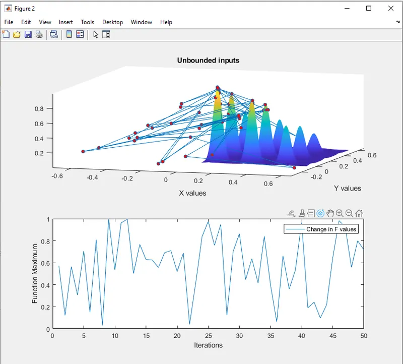
We are now plotting the different results of the genetic algorithm in a more complex plot. That is leading us to see that we are evaluating some results for some values that are outside the range, so not very useful. Eventhough we are beginning with the X and Y values between 0 and 0.6, the random effect of the genetic algorithm ended up getting values all over the place. We are using the command 'tic' and 'toc' for the first time. These are used to calculate the time is takes to exucutes the code in bewteen, and we are storing the value in second, in a variable.

% Study #1 - without boundaries
%timer on
tic
for i =1 : case_num
  [inputs,fval_opt(i)]=ga(@stalagmite,2);  
  xopt(i)=inputs(1);
  yopt(i)=inputs(2);
end
%timer off
study_1_time = toc

figure(2)
subplot(2,1,1)
hold on
surfc(xx,yy,-f)
shading interp
plot3(xopt,yopt,-fval_opt,'marker','o','markersize',5,'markerfacecolor','r')
xlabel('X values')
ylabel('Y values')
title('Unbounded inputs')

subplot(2,1,2)
plot(-fval_opt)
xlabel('Iterations')
ylabel('Function Maximum')
legend('Change in F values')

SECOND STUDY with defined boundaries :

We are now going to redo the same thing, but this time with boundaries. To achieve this, we are using an extra argument in the 'ga' command. This will run the algoirthm using values that are within the range specified. The values of x and y, will be between 0 and 1.

%timer on
tic
for i =1 : case_num
 [inputs,fval_opt(i)]=ga(@stalagmite,2,[],[],[],[],[0,0],[1,1]);  
  xopt(i)=inputs(1);
  yopt(i)=inputs(2);
end
%timer off
study_2_time = toc

figure(3)
subplot(2,1,1)
hold on
surfc(x,y,-f)
shading interp
plot3(xopt,yopt,-fval_opt,'marker','o','markersize',5,'markerfacecolor','r')
title('Unbounded inputs')
xlabel('X-values')
ylabel('Y-values')

subplot(2,1,2)
plot(-fval_opt)

xlabel('Iterations')
ylabel('Function Maximum')
legend('Change in F values')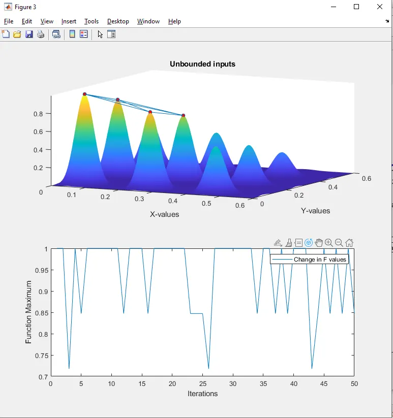

THIRD STUDY : increasing the number of 'ga' iterations

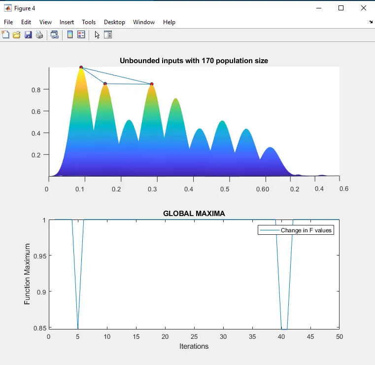
Due to the nature of the genetics algorithm, we have still a large number of possible fuction values. This could be due to our first initial population being too small. We will try again the genetic alogorithm with a larger number of iteration. We will specify an extra optional argument, 'PopulationSize'.Here the populatiom size of 170 is defined.

options = optimoptions('ga')
options = optimoptions(options,'PopulationSize',170);
tic
for i =1 : case_num
 [inputs,fval_opt(i)]=ga(@stalagmite,2,[],[],[],[],[0,0],[1,1],[],[],options);  
  xopt(i)=inputs(1);
  yopt(i)=inputs(2);
end
%timer off
study_3_time = toc

figure(4)
subplot(2,1,1)
hold on
surfc(x,y,-f)
shading interp
plot3(xopt,yopt,-fval_opt,'marker','o','markersize',5,'markerfacecolor','r')
title('Unbounded inputs with 170 population size')


subplot(2,1,2)
plot(-fval_opt)
title('GLOBAL MAXIMA');
xlabel('Iterations')
ylabel('Function Maximum')
legend('Change in F values')

FULL PROGRAM :

clear all 
close all 
clc 

%Preparing the data

%defining our search space
x = linspace(0,0.6,150);
y = linspace(0,0.6,150);

% number of times genetic algorithm going to run
case_num = 50;


%Creating a 2 dimension mesh
[xx,yy]= meshgrid(x,y);

%evaluating the stalagmite function
for i = 1:length(xx);
    for j = 1:length(yy);
        input_vector(1)=xx(i,j);
        input_vector(2)=yy(i,j);
        f(i,j) = stalagmite(input_vector);
    end
end

% plotting the graphic area
figure(1)
surfc(xx,yy,-f)
%axis identification
xlabel('X value')
ylabel('Y value')
zlabel('Z value')
title('GLOBAL MAXIMA');
legend('STALAGMITE','GLOBAL MAXIMA')
%removing the 3D grid lines
shading interp
colorbar

%Applying the genetics algorithm
[inputs,fval]=ga(@stalagmite,2,[],[],[],[],[0,0],[0.6,0.6])

%Optimization Studies

% Study #1 - without boundaries
%timer on
tic
for i =1 : case_num
  [inputs,fval_opt(i)]=ga(@stalagmite,2);  
  xopt(i)=inputs(1);
  yopt(i)=inputs(2);
end
%timer off
study_1_time = toc

figure(2)
subplot(2,1,1)
hold on
surfc(xx,yy,-f)
shading interp
plot3(xopt,yopt,-fval_opt,'marker','o','markersize',5,'markerfacecolor','r')
xlabel('X values')
ylabel('Y values')
title('Unbounded inputs')

subplot(2,1,2)
plot(-fval_opt)
xlabel('Iterations')
ylabel('Function Maximum')
legend('Change in F values')

% Study #2 - with defined boundaries
%timer on
tic
for i =1 : case_num
 [inputs,fval_opt(i)]=ga(@stalagmite,2,[],[],[],[],[0,0],[1,1]);  
  xopt(i)=inputs(1);
  yopt(i)=inputs(2);
end
%timer off
study_2_time = toc

figure(3)
subplot(2,1,1)
hold on
surfc(x,y,-f)
shading interp
plot3(xopt,yopt,-fval_opt,'marker','o','markersize',5,'markerfacecolor','r')
title('Unbounded inputs')
xlabel('X-values')
ylabel('Y-values')

subplot(2,1,2)
plot(-fval_opt)

xlabel('Iterations')
ylabel('Function Maximum')
legend('Change in F values')

% Study #3 - increasing the number of 'ga' iterations
options = optimoptions('ga')
options = optimoptions(options,'PopulationSize',170);
tic
for i =1 : case_num
 [inputs,fval_opt(i)]=ga(@stalagmite,2,[],[],[],[],[0,0],[1,1],[],[],options);  
  xopt(i)=inputs(1);
  yopt(i)=inputs(2);
end
%timer off
study_3_time = toc

figure(4)
subplot(2,1,1)
hold on
surfc(x,y,-f)
shading interp
plot3(xopt,yopt,-fval_opt,'marker','o','markersize',5,'markerfacecolor','r')
title('Unbounded inputs with 170 population size')


subplot(2,1,2)
plot(-fval_opt)
title('GLOBAL MAXIMA');
xlabel('Iterations')
ylabel('Function Maximum')
legend('Change in F values')

%end of the program

stalagmite function :

function [f] = stalagmite(input_vector)

x= input_vector(1);
y= input_vector(2);

f1 = (sin(5.1*pi*x + 0.5)).^6;
f2 = exp(-4*log(2)*((x-0.0667).^2)./0.64);
f3 = (sin(5.1*pi*y + 0.5)).^6;
f4 = exp(-4*log(2)*((y-0.0667).^2)./0.64);

f = -(f1*f2*f3*f4);

end

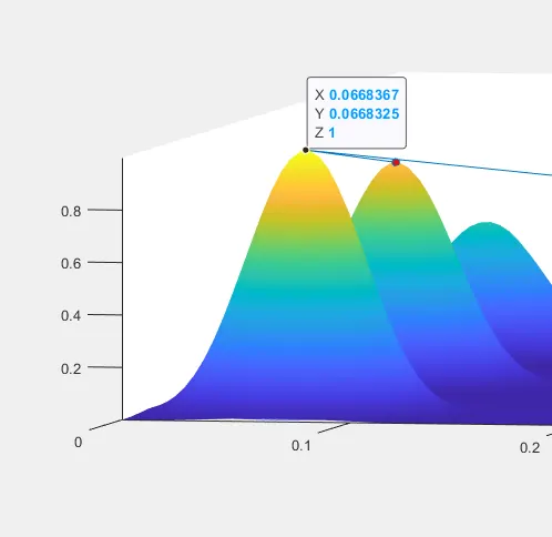
The 'Global Maxima' is 1 located at (0.0668367,0.0668325).

Study time for all three studies :

study_1_time =3.8796

study_2_time =5.0989

study_3_time =15.0015

ERRORS FACED :

ERROR 1 : Incorrect spelling leads to unrecognized function

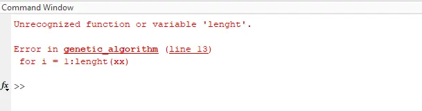
solved by changing the line with correct spelling

ERROR 2 : invalid index position2

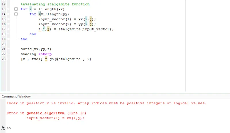
solved by replcaing "j" in place of "i" under the sub for loop.

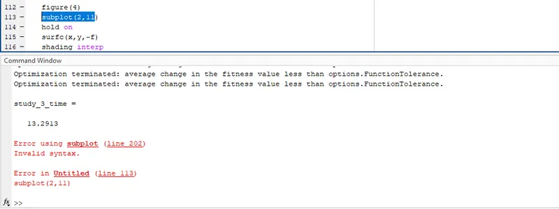
ERROR 3 : Error in positioning of sublot :

solved by seperating the row,column and position number of the plot with comma (,) i.e., subplot(2,1,1)

REFERENCES :

1. https://www.tutorialspoint.com/genetic_algorithms/genetic_algorithms_termination_condition.htm
2. https://in.mathworks.com/help/gads/how-the-genetic-algorithm-works.html
3. Introduction to Genetic Algorithms — Including Example Code | by Vijini Mallawaarachchi | Towards Data Science - https://towardsdatascience.com/introduction-to-genetic-algorithms-including-example-code-e396e98d8bf3#:~:text=A%20genetic%20algorithm%20is%20a,offspring%20of%20the%20next%20generation
4. Introduction to Optimization with Genetic Algorithm - KDnuggets