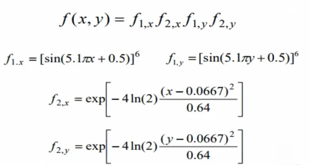
Week 4.1 - Genetic Algorithm

Code with comments:

clear all
close all
clc

% defining search space
x = linspace(0,0.6,150);
y = linspace(0,0.6,150);
num = 50;

% Creating a 2D mesh
[xx, yy] = meshgrid(x,y);

% evaluating the stalagmite function
for i = 1:length(xx)
    for j = 1:length(yy)
        input_vector(1) = xx(i,j);
        input_vector(2) = yy(i,j);
        f(i,j) = stalagmite(input_vector);
    end
end

% 3D plot
subplot (2,1,1)
surfc(xx,yy,-f)
xlabel('Iterations')
ylabel('Maximun Value')
shading interp
subplot(2,1,2)
plot(-f)
xlabel('Iterations')
ylabel('Maximun Value')

for i = 1:50
    
    [input_vector,fval(i)] = ga(@stalagmite,2);
end

% Case 1: statistical behaviour
for i = 1:num;
    [input_vector,output(i)] = ga(@stalagmite,2);
    xout(i) = input_vector(1);
    yout(i) = input_vector(2);
end

figure (2)
subplot(2,1,1)
surfc(xx,yy,-f)
shading interp
hold on 
plot3(xout,yout,-output)
title('unbounded plot')
subplot(2,1,2)
plot(-output)
xlabel('Iterations')
ylabel('Maximun Value')

% Case 2: Upper limit and lower limit behaviour
for i = 1:num;
    [input_vector,output(i)] = ga(@stalagmite,2,[],[],[],[],[0;0],[0.6;0.6],[],[]);
        xout(i) = input_vector(1);
        yout(i) = input_vector(2);
end

figure (3)
subplot(2,1,1)
surfc(xx,yy,-f)
shading interp
hold on 
plot3(xout,yout,-output)
title('Bounded plot')
subplot(2,1,2)
plot(-output)
xlabel('Iterations')
ylabel('Maximun Value')

% Case 3: Incereasing Population Size

option = optimoptions('ga','populationsize',250);

for i = 1:num;
    [input_vector,output(i)] = ga(@stalagmite,2,[],[],[],[],[0;0],[0.6;0.6],[],[],options);
        xout(i) = input_vector(1);
        yout(i) = input_vector(2);
end

figure (4)
subplot(2,1,1)
surfc(xx,yy,-f)
shading interp
hold on 
plot3(xout,yout,-output)
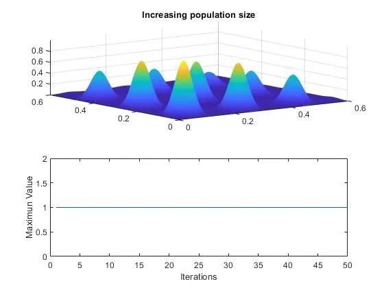
title('Increasing population size')
subplot(2,1,2)
plot(-output)
xlabel('Iterations')
ylabel('Maximun Value')

Outputs:

Figure 1:

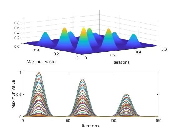
Figure 2 (for Case 1: statistical behaviour):

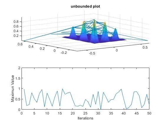
Figure 3 (for case 2: bounded limits):

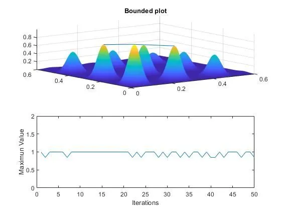
Figure 4 (for Case 3: Increase in population size):

Errors:

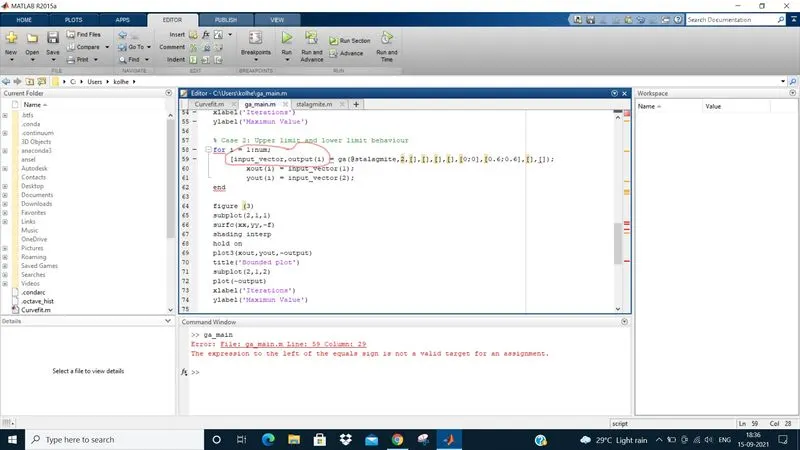
1.) The input array was not complete due to the missing of a closing parenthesis.

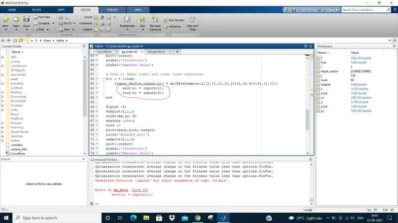
2.) The variables defined in for loop were not assigned to the variables assigned in the main code.

Explanation of ga:

A Genetic Algorithm is a code used to solve the constrained and unconstrained optimization problems.

There are 3 steps in which ga is done:

1. Selection: It selects the individuals called parents that contribute to the population in the next generation.

2. Crossover: It combines two parents to form the next generation.

3. Mutation: It randomly changes the individual parents to form the children.

The toolbox used to perform ga in Matlab is the Global Optimization Toolbox.

Syntax of ga is:

[x,fval] = ga(fun,x0,A,b,Aeq,beq,lb,ub,nonlcon,options)
it defines both upper limit and lower limit for x. If there is no linear equation then set the values Aeq=[] and beq=[]. 

To run the ga we need the governing function. its syntax is as below: