Project 2 - Rankine cycle Simulator

Code with comments:

% Main Code

clear all
close all
clc

% Displaying the Rankine cycle simulator:

disp (' Rankine cycle Simulator')
fprintf('\n 1-2 is the isentropic expansion process')
fprintf('\n 2-3 is the process of constant heat rejection')
fprintf('\n 3-4 is the isentropic compression process')
fprintf('\n 4-1 is the process of constant pressure heat addition')

% Variables for Stage 1:
p1 = 30;
t1 = 400;
h1 = XSteam('h_pT',30,400);
s1 = XSteam('s_ph',30,h1);

fprintf('\n	\nResults');
% fprintf('\n at state point 1');
fprintf('\n p1 is : %f bar',p1);
fprintf('\n t1 is : %f degree c',t1);
fprintf('\n h1 is : %f KJ/Kg',h1);
fprintf('\n s1 is : %f KJ/KgK',s1);

% Variables for state point 2:
p2 = 0.05;
s2 = s1;
t2 = XSteam('T_ps',0.05,6.1858);
sf2 = XSteam('sL_p',p2);
sg2 = XSteam('sV_p',p2);
hf2 = XSteam('hL_p',p2);
hg2 = XSteam('hV_p',p2);
x = ((s2 - sf2)/(sg2 - sf2));
h2 = hf2 + (x*(hg2 - hf2));
v2 = XSteam('v_ph',p2,h2);

fprintf('nn At state point 2');
fprintf('\n p2 is : %f bar',p2);
fprintf('\n t2 is : %f degree c',t2);
fprintf('\n h2 is : %f KJ/Kg',h2);
fprintf('\n s2 is : %f KJ/KgK',s2);

% Variables for State point 3:
t3 = t2;
p3 = p2;
s3 = XSteam('sL_p',p3);
h3 = XSteam('hL_T',32.875);
v3 = XSteam('v_ph',p3,h3);

fprintf('nn at State point 3');
fprintf('\n p3 is : %f bar',p3);
fprintf('\n t3 is : %f degree c',t3);
fprintf('\n h3 is : %f KJ/Kg',h3);
fprintf('\n s3 is : %f KJ/KgK',s3);

% variables for point 4:
s4 = s3;
p4 = p1;
v4 = v3;
h4 = XSteam('h_ps',p4,s4);
t4 = XSteam('T_hs',h4,s4);

fprintf('nn at state point 4');
fprintf('\n p4 is : %f bar',p4);
fprintf('\n t4 is : %f degree c',t4);
fprintf('\n h4 is : %f KJ/Kg',h4);
fprintf('\n s4 is : %f KJ/KgK',s4);

% variables for state variable 5:
p5 = p4;
t5 = XSteam('Tsat_p',p5);
h5 = XSteam('hL_T',t5);
s5 = XSteam('sL_p',p5);

fprintf('nn at state variable 5');
fprintf('\n p5 is : %f bar',p5);
fprintf('\n t5 is : %f degree c',t5);
fprintf('\n h5 is : %f KJ/Kg',h5);
fprintf('\n s5 is : %f KJ/KgK',s5);

% variables for stage 6:
t6 = t5;
p6 = XSteam('psat_T',t5);
s6 = XSteam('sV_T',t6);
h6 = XSteam('hV_T',t6);

fprintf('nn at state variable 6');
fprintf('\n p6 is : %f bar',p6);
fprintf('\n t6 is : %f degree c',t6);
fprintf('\n h6 is : %f KJ/Kg',h6);
fprintf('\n s6 is : %f KJ/KgK',s6);

% loops to find the variables on the saturation line:

t = linspace(0,400,1000);
for i=1:length(t)
	s_line1(i) = XSteam('sL_T',t(i));
end
for j = 1:length(t)
	s_line2(j) = XSteam('sV_T',t(j));
end

for i=1:length(t)
	h_line1(i) = XSteam('hL_T',t(i));
end
for j=1:length(t)
	h_line2(j) = XSteam('hV_T',t(j));
end

% final output :

w_turbine = h1-h2;	% work done by turbine
w_pump = h4-h3;		% work taken by pump
work = w_turbine-w_pump;	% net output
q_in = h1-h4;		% heat addition
q_out = h2-h3;		% heat rejection

% thermal efficiency:

n = work/q_in;

% backwork ratio:

bwr = w_pump/w_turbine;

% specific steam consumption:

ssc = 3600/work;

% graphs:
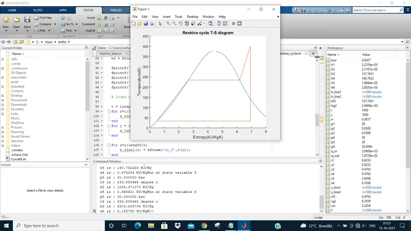
% 1.) T vs S graph
figure(1)
hold on;
plot([s_line1 s_line2],[t t]);
plot([s1 s2 s3 s4 s5 s6 s1],[t1 t2 t3 t4 t5 t6 t1]);
title('Rankine cycle T-S diagram');
xlabel('Entropy(KJ/KgK)');
ylabel('Temperature(K)');
axis([0,8,0,450]);

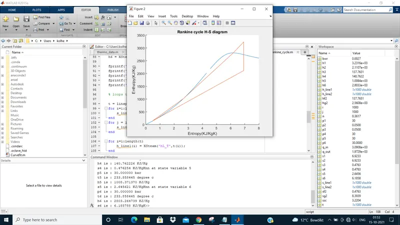
% 2.) H vs S graph
figure(2)
hold on;
plot([s_line1 s_line2],[h_line1 h_line2]);
plot([s1 s2 s3 s4 s5 s6 s1],[h1 h2 h3 h4 h5 h6 h1]);
title('Rankine cycle H-S diagram');
xlabel('Entropy(KJ/KgK)');
ylabel('Enthalpy(KJ/Kg)');
axis([0,8,0,3500]);

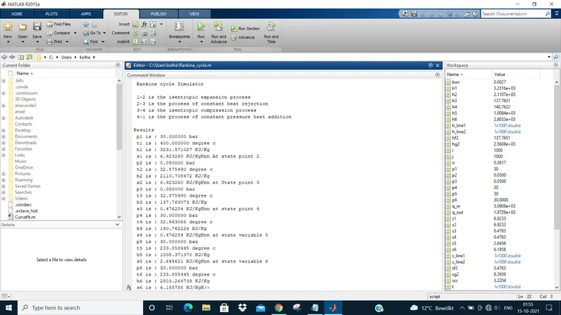
Outputs and results :

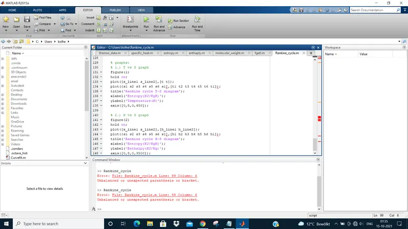
Errors:

1.) typo in defining variables

used h where t was supposed to be used

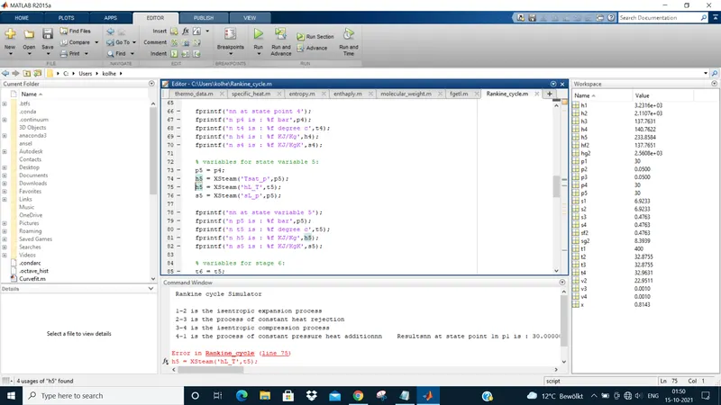
2.) wrong use of parenthesis

used curly braces instead of square.

My research about rankine cycle:

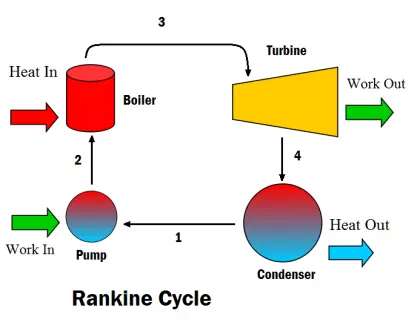
The Rankine cycle is an idealized thermodynamic cycle describing the process by which certain heat engines which allow mechanical work to be extracted from a fluid as it moves between a heat source and heat sink.

There are four stages in the Rankine cycle.

• Stage 1: The working fluid is pumped from low to high pressure. As the fluid is a liquid at this stage, the pump requires little input energy. Stage 1 is isentropic compression.
• Stage 2: The high-pressure liquid enters a boiler, where it is heated at constant pressure by an external heat source to become a dry saturated vapour. Stage 2 is constant pressure heat addition in boiler.
• Stage 3: The dry saturated vapour expands through a turbine generating power. This decreases the temperature and pressure of the vapour, and some condensation may occur. Stage 3 is isentropic expansion.
• Stage 4: The wet vapour then enters a condenser where it is condensed at a constant pressure to become a saturated liquid. Stage 4 is constant pressure heat rejection in condenser.

When the calculations are done manually or using a thermodynamic tables there are some variables which are:

	Heat flow rate to or from the system (energy per unit time)
	mass flow rate (mass per unit time)
	Mechanical power consumed by or provided to the system (energy per unit time)
	Thermodynamic efficiency of the process (net power output per heat input, dimensionless)
	Isentropic efficiency of the compression (feed pump) and expansion (turbine) processes, dimensionless
	The "specific enthalpies" at indicated points on the t vs s graph
	The final "specific enthalpy" of the fluid if the turbine were isentropic
	The pressures before and after the compression process

Formulas :

thermal efficiency = (W-thermal - W)/Qin

heat add = h1-h4

heat remove = h2-h3

workdone by turbine = h1-h2

workdone by pump = h4-h3

back work ratio = wpump/wturbine

net output = wturbine-wpump

References:

https://energyeducation.ca/encyclopedia/Rankine_cycle

wikipedia

https://www.nuclear-power.com/nuclear-engineering/thermodynamics/laws-of-thermodynamics/thermal-efficiency/thermal-efficiency-of-rankine-cycle/