Genetic Algorithm

AIM:

• To write a code in MATLAB to optimize the stalagmite function and find the global maxima of the function.

GA - Genetic Algorithm - Theory

A genetic algorithm is a search heuristic that is inspired by Charles Darwin’s theory of natural evolution. This algorithm reflects the process of natural selection where the fittest individuals are selected for reproduction in order to produce offspring of the next generation.

Five phases are considered in a genetic algorithm.

1. Initial population - The process begins with a set of individuals which is called a Population. Each individual is a solution to the problem you want to solve.
2. Fitness function - The fitness function determines how fit an individual is (the ability of an individual to compete with other individuals)
3. Selection - The idea of selection phase is to select the fittest individuals
4. Crossover - a crossover point is chosen at random and crossover between individuals happen until they reach the crossover point.
5. Mutation - Mutation occurs to maintain diversity within the population and prevent premature convergence.

For understanding:

If we want to determine the minimum drag of the race car, traditionally we will modify or changing various inputs and performing lots of combinations of inputs until we are supposed to get the desired output ie, minimum drag which will take a lot of time. But with genetic algorithm, we can determine the best combinations of inputs within less time.

Syntax

Stopping criteria

Exit Flag	Meaning
1	Without nonlinear constraints — Average cumulative change in value of the fitness function over MaxStallGenerations generations is less than FunctionTolerance, and the constraint violation is less than ConstraintTolerance.
	With nonlinear constraints — Magnitude of the complementarity measure (see Complementarity Measure) is less than sqrt(ConstraintTolerance), the subproblem is solved using a tolerance less than FunctionTolerance, and the constraint violation is less than ConstraintTolerance.
3	Value of the fitness function did not change in MaxStallGenerations generations and the constraint violation is less than ConstraintTolerance.
4	Magnitude of step smaller than machine precision and the constraint violation is less than ConstraintTolerance.
5	Minimum fitness limit FitnessLimit reached and the constraint violation is less than ConstraintTolerance.
0	Maximum number of generations MaxGenerations exceeded.
-1	Optimization terminated by an output function or plot function.
-2	No feasible point found.
-4	Stall time limit MaxStallTime exceeded.
-5	Time limit MaxTime exceeded.

STALAGMITE FUNCTION PROGRAM

%stalagmite function program
function [results] = stalagmite_func_practise(input_vector) 

x=input_vector(1); % assigned to x
y=input_vector(2); % assigned to y
f_1x= ((sin(5.1*pi*x+0.5)).^6);
f_1y= ((sin(5.1*pi*y+0.5)).^6);
f_2x= exp((-4*log(2)*((x-0.0667).^2./0.64)));
f_2y= exp((-4*log(2)*((y-0.0667).^2./0.64)));
% formula for creating stalagmite formation
[results] = -(f_1x.*f_2x.*f_1y.*f_2y); %- sign is used for inverting the graph (to find the maximum value x,y)
end

MAIN PROGRAM

%main program
clear all
close all
clc
%one dimensional
x=linspace(0,0.6,150); %x axis from 0 to 0.6 |150-values
y=linspace(0,0.6,150); %y axis from 0 to 0.6 |150-values
n=50;                  %number of itearation
A=[];         
b=[];         
Aeq=[];       
beq=[];       
lb=[0 0];              %lower bounds
ub=[0.6 0.6];          %upper bounds
nonlcon=[];   
Intcon=[];    
%2 d mesh
[xx,yy]=meshgrid(x,y); % converting into 2d grid plot

%for creating stalagmite plot
for i=1:length(xx)     
    for j=1:length(yy) 
        input_vector(1)=xx(i,j);   % xx(x,y)values inputed into input_vector(1)
        input_vector(2)=yy(i,j);   % yy(x,y)values inputed into input_vector(2)
        f(i,j)=stalagmite_func_practise(input_vector); % calling stalagmite function 
    end
end

%case 1
tic 
for k=1:n 
    [output,fval(k)]=ga(@stalagmite_func_practise,2); %genetic alogorithm | @function on which ga performed 
    %[output,fval(k),exitflag]=ga(@stalagmite_func_practise,2);
    xval(k)=output(1); 
    yval(k)=output(2); 
end
case_1=toc 

figure(1) 
subplot(2,1,1) 
hold on 
surf(x,y,-f) 
xlabel('x axis'); 
ylabel('y axis'); 
shading interp;    %removing grid on stalagmite graph for smoother look
plot3(xval,yval,-fval,'marker','o','markersize',5,'markerfacecolor','red'); 
title('unbounded outputs') 
subplot(2,1,2) 
plot(-fval) 
xlabel('iterations'); 
ylabel('maximum function');

%case 2:
tic
for k = 1:n
    [output, fval(k)]=ga(@stalagmite_func_practise,2,[],[],[],[],lb,ub); %with lower upper bounds
    %[output, fval(k),exitflag]=ga(@stalagmite_func_practise,2,[],[],[],[],lb,ub);
    xval(k)=output(1);
    yval(k)=output(2);
end
case_2=toc

figure(2)
subplot(2,1,1)
hold on
surf(x,y,-f)
xlabel('x axis');
ylabel('y axis');
shading interp;
plot3(xval,yval,-fval,'marker','o','markersize',5,'markerfacecolor','red');
title('bounded outputs') 
subplot(2,1,2)
plot(-fval)
xlabel('iterations');
ylabel('maximum function');

%case 3:
tic
options=optimoptions('ga','PopulationSize',170); % solver name | name | value

for k=1:n
    [output, fval(k)] = ga(@stalagmite_func_practise,2,[],[],[],[],lb,ub,[],[],options);% with bounds and options
    %[output, fval(k),exitflag] = ga(@stalagmite_func_practise,2,[],[],[],[],lb,ub,[],[],options);
    xval(k)=output(1);
    yval(k)=output(2);
end
case_3=toc

figure(3)
subplot(2,1,1)
hold on
surf(x,y,-f)
xlabel('x axis');
ylabel('y axis');
shading interp;
plot3(xval,yval,-fval,'marker','o','markersize',5,'markerfacecolor','red');
title('bounded outputs with increased population size')
subplot(2,1,2)
plot(-fval)
xlabel('iterations');
ylabel('maximum function');
       

Explanation

1.stalagmite function program

function [results] = stalagmite_func_practise(input_vector) function || arguments

x=input_vector(1); values from input_vector(1) is assigned to x
y=input_vector(2); values from input_vector(2) is assigned to y
f_1x= ((sin(5.1*pi*x+0.5)).^6);
f_1y= ((sin(5.1*pi*y+0.5)).^6);
f_2x= exp((-4*log(2)*((x-0.0667).^2./0.64)));
f_2y= exp((-4*log(2)*((y-0.0667).^2./0.64)));
% formula for creating stalagmite formation f_1x*f_1y*f_2x*f_2y
[results] = -(f_1x.*f_2x.*f_1y.*f_2y); '-' sign is used for inverting the graph (to find the maximum value x,y), since ga is used for only minimizing optimization
end

2.main program

%one dimensional
x=linspace(0,0.6,150); x axis from 0 to 0.6 |150-values
y=linspace(0,0.6,150); y axis from 0 to 0.6 |150-values
n=50; number of itearation
A=[]; linear inequalities A in Ax<=b
b=[]; linear inequalities b in Ax<=b
Aeq=[]; linear equalities A in Ax==b
beq=[]; linear equalities b in Ax==b
lb=[0 0]; lower bounds
ub=[0.6 0.6]; upper bounds
nonlcon=[]; nonlinear constraints
Intcon=[]; integer values

%2 d mesh
[xx,yy]=meshgrid(x,y); converting into 2d grid plot

%for creating stalagmite plot
for i=1:length(xx) from 1 to 150
for j=1:length(yy) from 1 to 150
input_vector(1)=xx(i,j); xx(x,y)values inputed into input_vector(1)
input_vector(2)=yy(i,j); yy(x,y)values inputed into input_vector(2)
f(i,j)=stalagmite_func_practise(input_vector); calling stalagmite function
end
end

%case 1
tic tic toc is used to measure the elapsed time
for k=1:n from 1 to 50 iterations
[output,fval(k)]=ga(@stalagmite_func_practise,2); genetic alogorithm | @function on which ga performed | number of variables(x,y)
%[output,fval(k),exitflag]=ga(@stalagmite_func_practise,2); included exitflag for finding the stopping creteria
xval(k)=output(1); 50 xval(k) values for determining fval(k)
yval(k)=output(2); 50 yval(k) values for determining fval(k)
end
case_1=toc elapsed time is stored in case_1

figure(1) figure 1
subplot(2,1,1) creating 2 X 1 grid(2-rows,1-column) || 1(first position graph)
hold on holding the figure
surf(x,y,-f) xx,yy f 3dimensional points(x,y,z)
xlabel('x axis'); labelled x axis
ylabel('y axis'); labelled y-axis
shading interp; removing grid on stalagmite graph for smoother look
plot3(xval,yval,-fval,'marker','o','markersize',5,'markerfacecolor','red'); plotting (x,y,z) points with o in red color
title('unbounded outputs') tittled as unbound outputs
subplot(2,1,2) creating 2 X 1 grid(2-rows,1-column) || 2(second position graph)
plot(-fval) plotting fvals for understanding
xlabel('iterations'); labelled as iterations
ylabel('maximum function'); labelled as maximum function

%case 2:
tic
for k = 1:n
[output, fval(k)]=ga(@stalagmite_func_practise,2,[],[],[],[],lb,ub); with lower upper bounds
%[output, fval(k),exitflag]=ga(@stalagmite_func_practise,2,[],[],[],[],lb,ub);
xval(k)=output(1);
yval(k)=output(2);
end
case_2=toc

figure(2)
subplot(2,1,1)
hold on
surf(x,y,-f)
xlabel('x axis');
ylabel('y axis');
shading interp;
plot3(xval,yval,-fval,'marker','o','markersize',5,'markerfacecolor','red');
title('bounded outputs') titled as bounded outputs
subplot(2,1,2)
plot(-fval)
xlabel('iterations');
ylabel('maximum function');

%case 3:
tic
options=optimoptions('ga','PopulationSize',170); solver name | name | value

for k=1:n
[output, fval(k)] = ga(@stalagmite_func_practise,2,[],[],[],[],lb,ub,[],[],options); with bounds and options
%[output, fval(k),exitflag] = ga(@stalagmite_func_practise,2,[],[],[],[],lb,ub,[],[],options);
xval(k)=output(1);
yval(k)=output(2);
end
case_3=toc

figure(3)
subplot(2,1,1)
hold on
surf(x,y,-f)
xlabel('x axis');
ylabel('y axis');
shading interp;
plot3(xval,yval,-fval,'marker','o','markersize',5,'markerfacecolor','red');
title('bounded outputs with increased population size') titled as boundes outputs with increased population size
subplot(2,1,2)
plot(-fval)
xlabel('iterations');
ylabel('maximum function');

Output plots with explanation

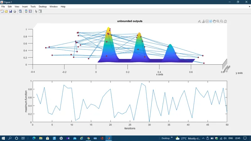
1. case-1 unbounded outputs - taking random values going beyond 0 and 0.6

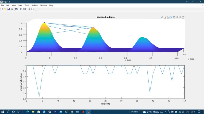
2. case-2 bounded outputs - smoother than case1, because of the lower and upper bounds [0 0] ,[0.6 0.6]

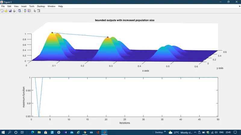
3. case-3 bounded outputs with increased population size - smother than case2, since we have increased the population size with bounded values. hence the probabilty of finding the maximum function for 50 iteration is almost flat with a single fluctuation as shown below.

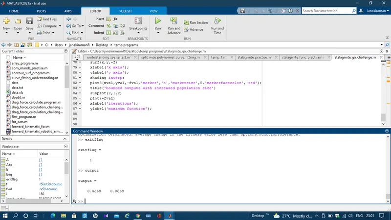
4. showing graphs with output - the output - 0.0668 0.0668 (will be same how much time we run the program)

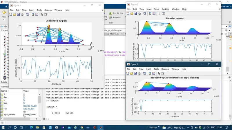
5. command window with exitflag value - 1 and message (Optimization terminated: average change in the fitness value less than options.FunctionTolerance.)

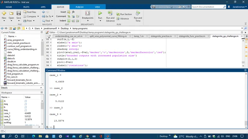
6. command window with time elapsed for all 3 cases - case 3 takes more time than the other cases because of the increase in population size.

References:

1. https://in.mathworks.com/help/gads/ga.html

2. https://in.mathworks.com/help/optim/ug/optim.problemdef.optimizationproblem.optimoptions.html

3. https://towardsdatascience.com/introduction-to-genetic-algorithms-including-example-code-e396e98d8bf3

4. youtube - stalagmite concept, global ,local - minimas and maximas.