Week 4.1 - Genetic Algorithm

1. Code for optimising the Stalagmite function and finding the Global maxima and minima

Step 1: Clearing the previous output from the screen and defining the search space using linspace command

clear all
close all
clc

%defining our search space
x = linspace(0,0.6,150);
y = linspace(0,0.6,150);
iterations = 50;

Explanation: The linspace command is used to set 150 different values forr x & y in between 0 & 0.6

Step 2: Creating a mesh - 2-D

%creating a 2-D mesh
[xx yy] = meshgrid(x,y);

Explanation : From the existing values of X & Y a 2-D mesh is created using the meshgrid Command

Step 3: Evaluating the Stalagmite Function

%evaluating the stalagmite function
for i=1:length(xx)
    for j = 1:length(yy)
        input_vector(1) = xx(i,j);
        input_vector(2) = yy(i,j);
        f(i,j) = stalagmite(input_vector);
    end
end

Explanation: The values of xx and yy are passed on to input vectors using for loop and then used to pass as arguments to stalagmite function

Step 4: Study 1 - Without any boundary conditions

tic
%study 1 without boundary conditions
for i = 1: iterations
    [inputs, fopt(i)] = ga(@stalagmite,2);
    
    xopt(i) = inputs(1);
    yopt(i) = inputs(2);
    
end

study1_time = toc;

Explanation: The tic & toc are used to calculate the amount of time taken by the function.

Step 5: Plotting for Study 1

figure(1)
subplot(2,1,1)
hold on 
surfc(x,y,f)
xlabel('x value')
ylabel('y value')
shading interp
plot3(xopt,yopt,fopt,'marker','o','markersize',5,'markerfacecolor','r')
title('NO BOUNDARY CONDITIONS - OUTPUT')
subplot(2,1,2)
plot(fopt)
xlabel('Iterations')
ylabel('Function Minimum')

Step 6: Study 2 with upper and lower Boundaries

%Study 2 - with upper and lower limits
tic
for k = 1: iterations
    [inputs, fopt(k)] = ga(@stalagmite,2,[],[],[],[],[0;0],[1;1]);
    xopt(k) = inputs(1);
    yopt(k) = inputs(2);
end
study2_time = toc;

Step 7 : Plotting for Study 2

figure(2)
subplot(2,1,1)
hold on
surfc(x,y,f)
xlabel('x value')
ylabel('y value')
shading interp
plot3(xopt,yopt,fopt,'marker','o','markersize',5,'markerfacecolor','r')
title('With upper and lower limits')
subplot(2,1,2)
plot(fopt)
xlabel('Iterations')
ylabel('Function Minimum')

Step 8: Study 3 - By increasing Population size Increasing the iterations

%Study 3 Increasing GA iterations by increasing population size to more
%than 50

options = optimoptions('ga');
options = optimoptions(options,'PopulationSize',170);

tic
for l = 1:iterations
    [inputs, fopt(l)] = ga(@stalagmite,2,[],[],[],[],[0:0],[1:1],[],[],options);
    xopt(l) = inputs(1);
    yopt(l) = inputs(2);
end    
study3_time = toc;

Step 9: Plotting for Study 3

figure(3)
subplot(2,1,1)
hold on
surfc(x,y,f)
xlabel('x value')
ylabel('y value')
shading interp
plot3(xopt,yopt,fopt,'marker','o','markersize',5,'markerfacecolor','r')
title('Increasing Population Method')
subplot(2,1,2)
plot(fopt)
xlabel('Iterations')
ylabel('Function Minimum')

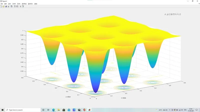
Step 9 : Final Surface plot from xx & yy values

figure(4)
surfc(xx,yy,f)
xlabel('x value')
ylabel('y value')

shading interp

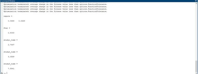
Step 10: Finding the time taken for each study

[inputs, fval] = ga(@stalagmite, 2,[],[],[],[],[0:0],[1:1],[],[],options)

study1_time,study2_time,study3_time

Step 11: STalagmite Function Definition

function [f] = stalagmite(input_vector)
x =input_vector(1);
y = input_vector(2);

f1_x = (sin(5.1*pi*x + 0.5)).^6;
f1_y = (sin(5.1*pi*y + 0.5)).^6;
f2_x = exp(-4*(log(2))*(((x-0.06670).^2)/0.64));
f2_y = exp(-4*(log(2))*(((y-0.06670).^2)/0.64));

g = f1_x * f2_x * f1_y * f2_y;
f = 1/(1+g);
end

Explanation: Firstly the values are transferred to the local variables x & y. Then using the Formulae defined for each values of f1,x;f1,y;f2,x;f2,y are calculated.

NO ERRORS FACED.
Output:

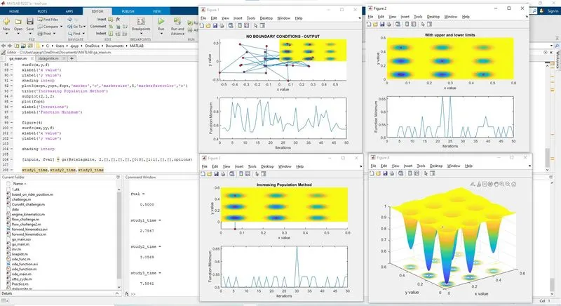
STUDY 1 OUTPUT:

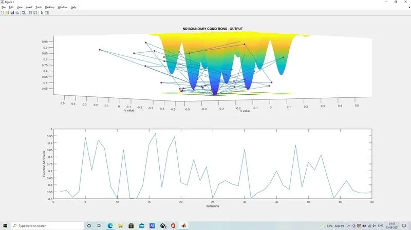
STUDY 2 OUTPUT:

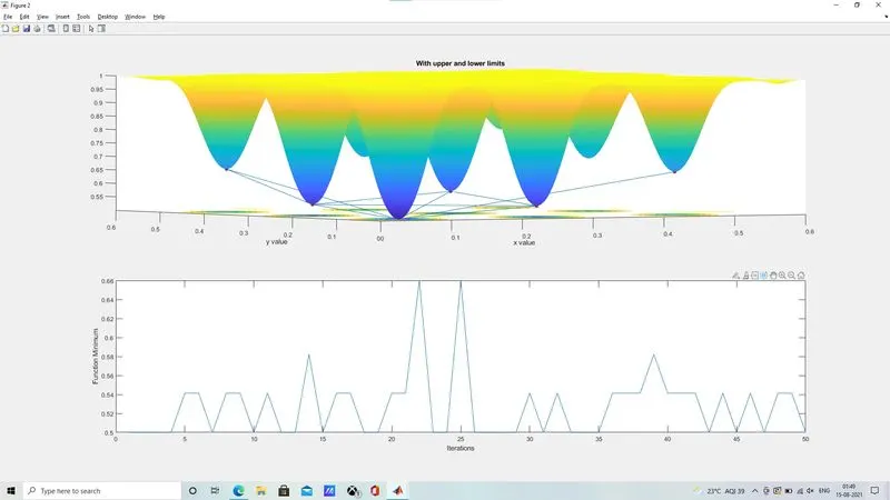
STUDY 3 OUTPUT:

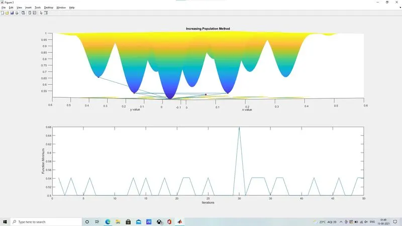
FINAL FIG OUTPUT:

VALUES OF STUDY TIME:

2.SYNTAX & EXPLANATION:

A GENETIC ALGORITHM is an algorithm created to find the best possible fitness or to predict the best possible chromosome that could be passed on to the next generation.

There are 8 steps involved in making a GA. They are as follows:

1. Finding the number of chromosomes that are worked on, the mutation rate , the number of generations for which the value is to be selected and the crossover rate values.

2. Generating the Values of Chromosome and Chromosome population,initializing the genes with random values for chromosomes

3. Evaluate the fitness values using a function

4. Select the chromosomes with best possible fitness

5. Crossover position determination

6. Mutation based on the number of generations

7. Repeat steps 3 to 6

8. Solution is made from the best chromosomes

GENERALLY USED SYNTAX IN GA:

1. x = ga(fun,nvars) finds a local unconstrained minimum, x, to the objective function, fun. nvars is the dimension (number of design variables) of function.

2. x = ga(fun,nvars,A,b) finds a local minimum x to fun, subject to the linear inequalities A*x ≤ b. ga evaluates the matrix product A*x as if x is transposed (A*x').