Week 4.1 - Genetic Algorithm
AIM- To perform coding operations in GENETIC ALGORITHM.
INTRODUCTION AND EQUATIONS- Genetic algorithms can be defined as the method for solving the various complex search and optimization problems. Genetic algorithms work on the concept of genetics and natural selection to provide solutions to problems by building a population of chromosomes which is a set of possible solutions to the optimization problem. Within a generation of a population, the chromosomes are randomly combine in order to create new chromosomes that have better evaluation scores.
- Selection select the individuals or (solutions), called parents, that contribute to the population at the next generation.
- Crossover combine two parents or (solutions) to form children or (better solutions) for the next generation.
- Mutation apply random changes to individual parents or (solutions) to form children.
There are many advantages of genetic algorithms over traditional optimization algorithms. Two most important are-
- The ability of dealing with complex problems and parallelism.
- Genetic algorithms can deal with various types of optimization, whether the objective (fitness) function is stationary or non-stationary (change with time), linear or nonlinear, continuous or discontinuous, or with random noise.
Because multiple offsprings in a population act like independent agents, the population (or any subgroup) can explore the search space in many directions simultaneously. This feature makes it ideal to parallelize the algorithms for implementation. Different parameters and even different groups of encoded strings can be manipulated at the same time.
Syntax for G.A.-
- x = ga(fun,nvars,A,b,Aeq,beq,lb,ub,nonlcon,options) minimizes with the default optimization parameters replaced by values in options. (Set nonlcon=[] if no nonlinear constraints exist.) Create options using optimoptions.
- x = ga(fun,nvars,A,b,[],[],lb,ub,nonlcon,IntCon) or x = ga(fun,nvars,A,b,[],[],lb,ub,nonlcon,IntCon,options) requires that the variables listed in IntCon take integer values.
- x = ga(problem) finds the minimum for problem, a structure described in problem.
- [x,fval,exitflag,output,population,scores] = ga(___) also returns a matrix population, whose rows are the final population, and a vector scores, the scores of the final population.
Optimization helps to deal with the way to minimize or maximize the particular solutions that depends on the input parameters.
OBJECTIVE-
- To write a code in MATLAB to optimise the stalagmite function and to find the global maxima of the function.
- To plot the graphs for all the 3 studies and for F maximum vs no. of iterations.
MAIN CONTENTS- Stalagmite Function- To create the function file stalagmite for the given problem statement-
%Writing the code for the given formulae
function[f] = stalagmite(input_vector)
x=input_vector(1);
y=input_vector(2);
fx1=(sin(5.1*pi*x+0.5)).^6
fy1=(sin(5.1*pi*y+0.5)).^6
fx2=exp(-4*log(2).*(((x-0.0667).^2)/0.64))
fy2=exp(-4*log(2).*(((y-0.0667).^2)/0.64))
%Multiplying all the above values with negative sign in order to get the global maxima
f=-(fx1*fx2*fy1*fy2)
end
Now from the above, a function is created as stalagmite which will be called in the below main code-
clear all
close all
clc
%Defining the search space for the given problem
x=linspace(0,0.6,140);
y=linspace(0,0.6,140);
%Converting x and y variables from 1D to 2D array
[xx,yy]=meshgrid(x,y);
%Using loop to create create the 3D plots
for i=1:length(xx)
    for j=1:length(yy)
        input_vector(1) = xx(i,j);
        input_vector(2) = yy(i,j);
        f(i,j)=stalagmite(input_vector);
    end
end
%Number of iterations
num_cases=50;
tic
%STUDY 1= Statistical Behaviour
for i=1:num_cases
    [inputs,fopt1(i)]=ga(@stalagmite,2)
    xopt1(i)=inputs(1);
    yopt1(i)=inputs(2);
end
%To calculate the evaluation time for STUDY 1
study1_time=toc
%To create both the plots in one figure
figure(1)
subplot(2,1,1)
hold on
colorbar
surfc(x,y,-f)
%To hide the grid lines
shading interp
xlabel('X DATA')
ylabel('Y DATA')
axis([0 0.6 0 0.6])
plot3(xopt1,yopt1,-fopt1,'marker','o','markersize',5,'markerfacecolor','b')
title('Unbounded Inputs')
subplot(2,1,2)
plot(-fopt1)
xlabel('Iterations')
ylabel('Function maximum')


tic
%STUDY 2=Statistical behaviour(with upper and lower bounds)
%Stalagmite function evaluation by setting the boundaries
for i=1:num_cases
    [inputs,fopt2(i)]=ga(@stalagmite,2,[],[],[],[],[0;0],[1;1]);
    xopt2(i)=inputs(1);
    yopt2(i)=inputs(2);
end
%To calculate the evaluation time for STUDY 2
study2_time=toc
figure(2)
%To create both the plots in second figure
subplot(2,1,1)
hold on
colorbar
surfc(x,y,-f)
%To hide the grid lines on the 3D plot
shading interp
xlabel('X DATA')
ylabel('Y DATA')
plot3(xopt2,yopt2,-fopt2,'marker','o','markersize',5,'markerfacecolor','g')
title('Bounded Inputs')
subplot(2,1,2)
plot(-fopt2)
xlabel('Iterations')
ylabel('Function maximum')


%STUDY 3=Increasing the additional parameters by varying population in GA
options=optimoptions('ga');
options=optimoptions(options,'Populationsize',150);
tic
for i=1:num_cases
    [inputs,fopt3(i)]=ga(@stalagmite,2,[],[],[],[],[0;0],[1;1],[],[],options);
    xopt3(i)=inputs(1);
    yopt3(i)=inputs(2);
end
%To calculate the evaluation time for STUDY 3
study3_time=toc
figure(3)
%To create the both the plots on third figure
subplot(2,1,1)
hold on
colorbar
surfc(x,y,-f)
%To hide the grid lines on the 3D plot
shading interp
xlabel('X DATA')
ylabel('Y DATA')
plot3(xopt3,yopt3,-fopt3,'marker','o','markersize',5,'markerfacecolor','r')
title('Bounded Inputs with modified population size')
subplot(2,1,2)
plot(-fopt3)
xlabel('Iterations')
ylabel('Function maximum')
OUTPUTS-
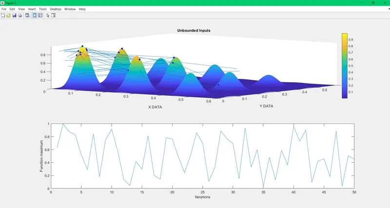
STUDY 1 OUTPUT-
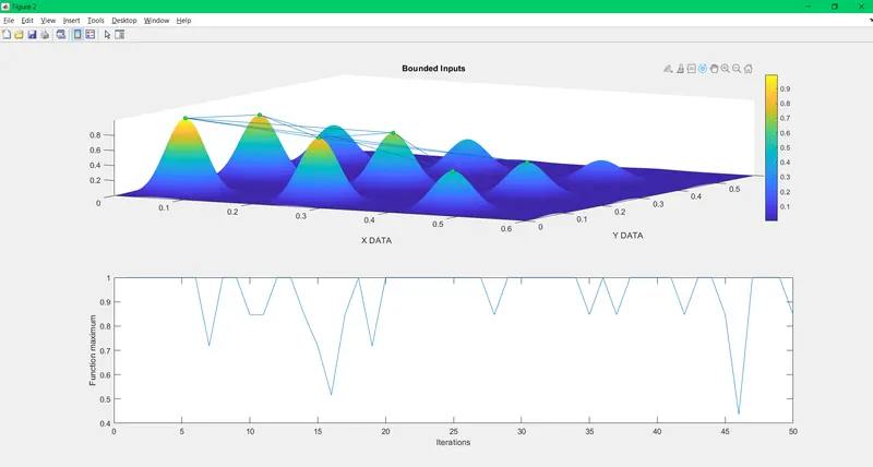
STUDY 2 OUTPUT-
STUDY 3 OUTPUT-
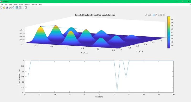
From the above 3 plots it is clear that by increasing the population size the value of global maxima is getting much more clear and accurate, this is because on every study the ga syntax has been modifying to get the better values of f that lies under the limit of x and y.
ERRORS FACED WHILE CODING-
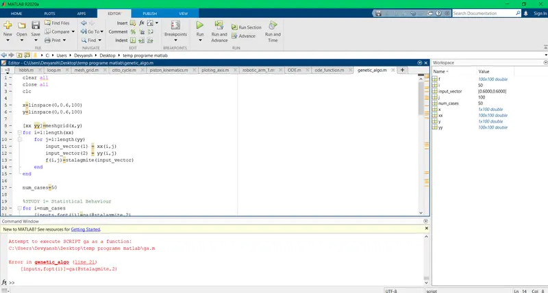
To overcome this error different opt values were taken for different case studies-
For eg.- For case study 1- opt1 was considered everywhere.
For case study 2- opt2 was considered everywhere.
For case study 3- opt3 was considered everywhere.
REFERENCES-