To plot the Otto cycle using MATLAB

AIM- To make an Otto cycle plot.

INTRODUCTION AND GOVERNING EQUATIONS- The Otto cycle is the theoretical cycle that is considered for reciprocating spark ignition engines. The four-stroke Otto cycle consists 4 internally reversible processes: 1–2 (isentropic compression) ; 2–3 (constant-volume heat addition) ; 3-4 (isentropic expansion) ; and 4–1 (constant-volume heat rejection). The actual exhaust and intake stroke has been replaced by process 4–1.

Representation of the Otto cycle-

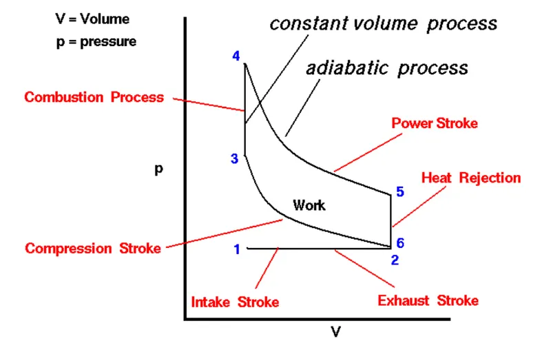
The isentropic equations of ideal gases and the constant pressure/volume relations for the process 1 to 2 and 3 to 4-

`(T2)/(T1)=((P2)/(P1))^((gamma-1)/gamma`

And, `(T2)/(T1)=((V1)/(V2))^(gamma-1)`

Where, `gamma=(C_p)/(C_v)`

`gamma` is the specific heat ratio

Swept volume= π/4*(bore)²*stroke

Clearance volume= Swept volume/(cr-1)

Where cr is the compression ratio

OBJECTIVE- To make a P-V plot of an Otto cycle and to find the thermal efficiency of the engine.

BODY OF THE CONTENT- 1. CODE SAMPLE-

clear all
close all
clc

%inputs based on standard general values
gama=1.4
cr=8

%engine parameters based on assumed existed values
b=0.1
s=0.1
con_rod=0.15
t3=2300

%process 1 variables
p1=101325
t1=500
t4=t1 

%calculation of swept and clearance volume
s_v=(pi/4)*b^2*s
c_v=s_v/(cr-1)
v1=s_v + c_v
v2=c_v 

const=p1*v1^gama
volume_com= piston_kinematics(b,s,con_rod,cr,180,0)
pressure_com=const./volume_com.^gama

%process 2 variables
%p2v2^gama=p1v1^gama
%p2=p1(v1/v2)^gama=p1*cr^gama
p2=p1*cr^gama
%p1v1/t1=p2v2/t2 // t2=t1*p2*v2/(p1*v1)
t2=t1*p2*v2/(p1*v1)


%process 3 variables
v3=v2
%p3v3/t3=p2v2/t2 // p3=t3*p2*v2/(t2*v3)
p3=t3*p2*v2/(t2*v3)

const=p3*v3^gama
volume_ex= piston_kinematics(b,s,con_rod,cr,0,180)
pressure_ex=const./volume_ex.^gama

%process 4 variables
v4=v1
%p3v3^gama=p4v4^gama | p4=p3*(v3/v4)^gama
p4=p3*(v3/v4)^gama

%Plotting the Otto cycle
hold on
plot([v1 v2 v3 v4],[p1 p2 p3 p4],'*','color','b','linewidth',2)
plot(volume_com,pressure_com,'color','b','linewidth',2)
plot(volume_ex,pressure_ex,'color','b','linewidth',2)
plot([v2 v3],[p2 p3],'color','r','linewidth',2)
plot([v4 v1],[p4 p1],'linewidth',2)

%To find out the thermal efficiency
thermal_efficiency=1-((t4-t1)/(t3-t2))

Code sample of the called FUNCTION - piston_kinematics-

function[volume]= piston_kinematics(bore,stroke,con_rod,cr,start_cr_angle,end_cr_angle)
 
 R=(2*con_rod)/stroke
 s_v=pi/4*bore^2*stroke
 c_v=s_v/(cr-1)
 theta=linspace(start_cr_angle,end_cr_angle,14000)
 term1=0.5.*(cr-1)
 term2=R+1-cosd(theta)
 term3=(R^2-sind(theta).^2).^0.5
 volume=c_v.*(1+term1*(term2-term3))

end

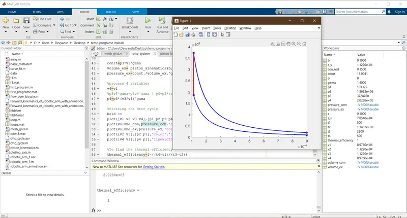
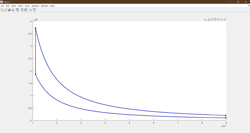
2. OUTPUT-

3. Errors faced while programming-

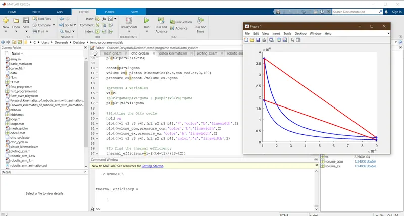
(The above image also signifies the differentiation between theoretical and actual OTTO cycle)

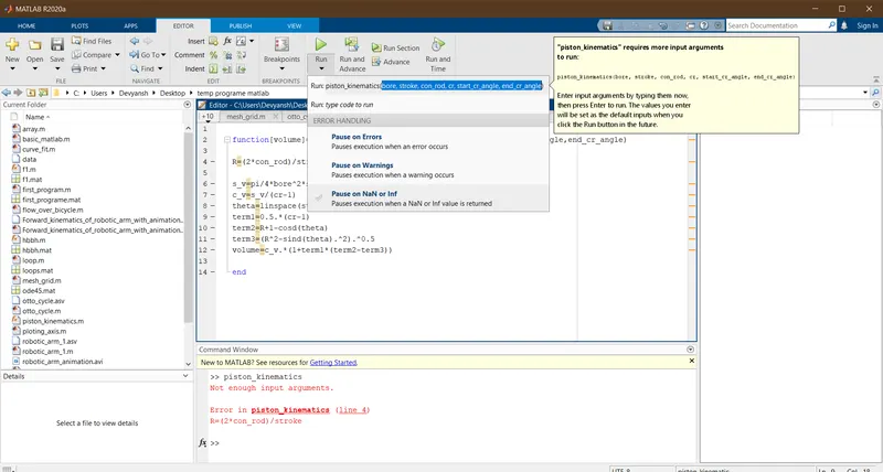
(The above mistake is common among newers as to check the function you need to call the function in the command window with exact name and then input the values accordingly)

CONCLUSION- The conclusion drawn is that it is much easier to generate any air standard cycle through MATLAB and it also gives the glimpse that how all those air standard cycles actually look on real parameters.