Week 4.1 - Genetic Algorithm
AIM : To write a code n Matlab to optimise the stalagmite function and find the global maxima of the function.
THEORY :
GENETIC ALGORITHM(GA): It is a method which mimics the principle used by Charles Darwin who made a theory to predict the natural biological evolution, to optimise constrained and unconstrained problems. The genetic algorithm uses concept of selecting random items from the population and slects them as "parents" to find "children" such that the parents undergo optimisation and evolution over successive "generations". The genetic algorithm can be used to optimise problems where the objective function is discontinous,highly non linear etc. which are difficult to be solved by standard algorithms.
SOME TERMS RELATED TO GENETIC ALGORITHM:
- Fitness function: function which has to be optimised using genetic algorithm.
- Individuals: any point to which fitness function can be applied.
- Population: Array of individuals is called population.
- Diversity: average distance between the individuals.
- Fitness values: value of the fitness function for an individuals.
- Best fitness function: The best fitness value of a of a population for any individual in the population
STALAGMITE FUNCTION:
The key equations used to define the stalagmite function:
f(x,y)=f1x*f2x*f1y*f1y*f2y;
`f1x=[sin(5.1pix+0.5)]^6`
`f1y=[sin(5.1piy+0.5)]^6`
`f2x=exp[(-4ln(2)(x-0.0667)^2/0.64)`
`f2y=exp[(-4ln(2)(y-0.0667)^2/0.64]`
CODE :
- Function used to define the stalagmite function
function [ fxy ] = stalagmite_function( inputs )
x=inputs(1);
y=inputs(2);
f1x=[sin(5.1*pi*x+0.5)]^6;
f1y=[sin(5.1*pi*y+0.5)]^6;
f2x= exp((-4*log(2))*((x-0.0667)^2)/0.64);
f2y= exp((-4*log(2))*((y-0.0667)^2)/0.64);
% Genetic algorithm finds the global minima of a function
% Hence to find maximum value we change sign of the function and hence the
% global maxima value is negative of the value found by GA for the negative
% function.
fxy= -(f1x*f1y*f2x*f2y);


end
2. Using genetic algorithm to optimise the function
% Finding maximum value of stalagmite function using genetic algorithm
x=linspace(0.0,0.6,250);
y=linspace(0.0,0.6,250);
n_iterations=100;
% Generating a 2 D Mesh
[xx,yy]=meshgrid(x,y);
% Evaluating the stalagmite function
for i=1:length(xx);
 for   j=1:length(yy);
     inputvector(1)=xx(i,j);
     inputvector(2)=yy(i,j);
     f(i,j)=stalagmite_function(inputvector);
 end
end
%% CASE I Statistical testing for unbounded constraints
tic % finding time required for the iteration
for i=1:n_iterations
    [inputs,fval(i)]=ga(@stalagmite_function,2); % syntax for genetic algorithm
    xopt(i)=inputs(1);
    yopt(i)=inputs(2);
end
    fval_case1=-fval;
    time1=toc
    % Plotting
    figure(1)
    subplot(2,1,1)
    surfc(xx,yy,-f) % creating 3 D plot of the stalagmite function
    xlabel('x input')
    ylabel('y input')
    shading interp
    hold on
    plot3(xopt,yopt,fval_case1,'marker','o','markersize',6,'markerfacecolor','r') % plotting maximas found by ga
    subplot(2,1,2)
    plot(-fval,'linewidth',3) % plotting variation of fitness values with no. of iterations
    axis([0 100 0 1.4])
    xlabel('iterations')
    ylabel('Fitness values')
    %% CASE II Statistical testing for bounded constraints with default population
    tic
for i=1:n_iterations
    [inputs,fval(i)]=ga(@stalagmite_function,2,[],[],[],[],[0;0],[0.6;0.6]);% ga syntax for bounded constraints
    xopt2(i)=inputs(1);
    yopt2(i)=inputs(2);
end
    fval_case2=-fval;
    time2=toc
    figure(2)
    subplot(2,1,1)
    surfc(xx,yy,-f)
    xlabel('x input')
    ylabel('y input')
    shading interp
    hold on
    plot3(xopt2,yopt2,fval_case2,'marker','o','markersize',6,'markerfacecolor','r')
    subplot(2,1,2)
    plot(-fval,'linewidth',3)
    axis([0 100 0 1.4])
    xlabel('iteration')
    ylabel('Fitness value')
    %% CASE III Statistical testing for bounded constraints with population 150
    % Changing the population size from default to 150
    options=optimoptions('ga');
    options=optimoptions(options, 'populationsize',150);
    tic
for i=1:n_iterations
    [inputs,fval(i)]=ga(@stalagmite_function,2,[],[],[],[],[0;0],[0.6;0.6],[],[],options);
    xopt3(i)=inputs(1);
    yopt3(i)=inputs(2);
end
fval_case3=-fval;
time3=toc
figure(3)
subplot(2,1,1)
surfc(xx,yy,-f)
xlabel('x input')
ylabel('y input')
hold on
plot3(xopt3,yopt3,fval_case3,'marker','o','markersize',6,'markerfacecolor','r')
subplot(2,1,2)
plot(-fval,'linewidth',3)
axis([0 100 0 1.4])
xlabel('iterations')
ylabel('fitness values')
%% CASE IV Statistical testing for bounded conditions with population 1000
% Changing the population size from default to 1000
options=optimoptions('ga');
options=optimoptions(options,'PopulationSize',1000);
tic
for i=1:n_iterations
    [inputs,fval(i)]=ga(@stalagmite_function,2,[],[],[],[],[0;0],[0.6;0.6],[],[],options);
    xopt4(i)=inputs(1);
    yopt4(i)=inputs(2);
end
fval_case4=-fval;
figure(4)
subplot(2,1,2)
surfc(xx,yy,-f)
xlabel('x input')
ylabel('y input')
hold on
plot3(xopt4,yopt4,fval_case4,'marker','o','markersize',6,'markerfacecolor','r')
subplot(2,1,2)
plot(-fval,'linewidth',3)
axis([0 100 0 1.2])
xlabel('iterations')
ylabel('fitness values')
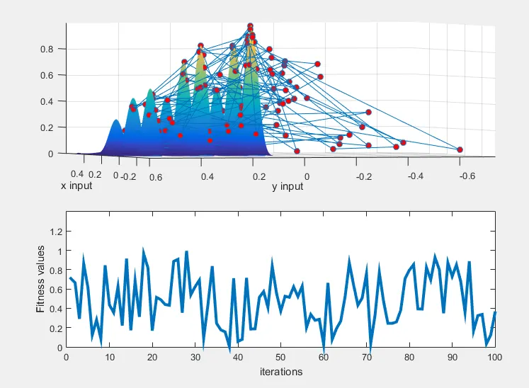
Fig 1 optimisaion with Unbounded constraints population size 50
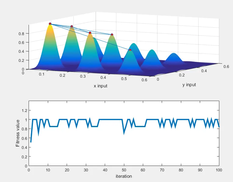
Fig 2 optimisation with bounded constraint population size of 50
WORKFLOW :
- A function code is written to define the stalagmite function which has to be optimised.
- Then code script is written to statistically analyse the optimisation using genetic algorithm
- The code is divided into four parts, to analyse the optimisation:
- fisrts case is for unbounded constarints with default population size of 50.
- second case is for bounded constraints with default population size of 50.
- third case is for bounded constarints with population size increased to 150.
- fourth case is for bounded constraints with population size increased to 1000.
RESULTS :
- The results for unounded constraints are least accurate but optimisation time is less.
- The more the accurate results the more is the time taken.
ERRORS FACED :
There were only few typing errors which were corrected instantaneously when detected.
REFERENCES :