Week 3 - Solving second order ODEs

AIM : Writing a program in Matlab to simulate the pendulum motion.

THEORY : The motion of a simple pendulum can be described with the help of Newton's second law. After apllying Newton's second law to its motion, a second order differential equations is easily devoloped. The derivation of second order differential equation that governs the motion of the simple pendulum is explained below.

DERIVATION OF THE SECOND ORDER DIFFERENTIAL EQUATION GOVERNING A SIMPLE HARMONIC MOTION

From Hookes law one can say that the restoring force is the function of the displacement and acts in the opposite direction.Also Newton's second law says that the magnitude of the force is mass times the accelration.

this implies, F=ma = -kx where k is the constant of proportionality

a can be written as the double derivative of the distance i.e. `d^2`x/`dt^2`=a

For real world oscillating systems damping also plays a role. Damping is the resistance offered to the oscillating system. Hence a damping force or frictional force is also present in the opposite direction of the motion of the oscillating object. This force is proportional to the velocity of the object.

Hence a simple second order differential equation can be derived by balancing the forces:

m `(d^2x)/dt^2`+kx+b`dx/dt`=0; where 'b' is the damping coefficient with units Ns/m or kg/s

GOVERNING EQUATION FOR A SIMPLE PENDULUM

We consider a simple pendulum with a spherical bob of mass 'm' attached to a string of length 'l' and negligible mass. At any time 't' it has angular displacement `theta`with respect to mean position(`theta`=0) as shown in the figure given below

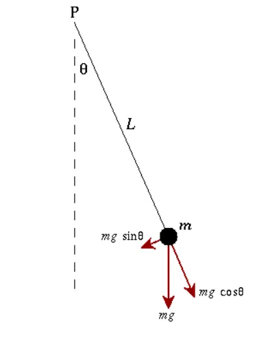
Fig 1. A simple pendulum free body diagram(image courtesy:https://www.acs.psu.edu/drussell/Demos/Pendulum/Pendulum.html)

From the figure above we can easily tell the restoring force is mg sin`theta` and hence the restoring torque is mgl sin`theta`.

therefore balancing torque we get

I`alpha`+mgl sin`theta`+ bl `(d theta)/dt`=0; where `alpha` is the angular acceleration

I is the moment of inertia of the pendulum and is m*`l^2`.

Hence by simplifying the final equation we get is

`(d^2theta)/dt + g/l sintheta + b/m (d theta)/dt = 0`;

OBJECTIVES OF THE REPORT :

The objective of the report is to write a Matlab code to :

1. Solve the above equation which is a second order ODE governing motion of a simple pendulum with given inputs
2. simulate the video with the help of Matlab describing motion of the pendulum

WORKFLOW :

A.)First we start from the given input conditions and initial conditions for the pendulum:

1. The length of the pendulum 'l' = 1m/s;
2. The mass of the pendulum 'm'= 1kg;
3. The damping coefficient 'b'= 0.05kg/s;
4. the gravitational constant 'g'=9.81m/`s^2`
5. initial conditions: angular displacement (at t=0)=0; angular velocity(at t=0)=3rad/s

B.)Writing code in Matlab using 'ode45' solver to solve the second order ODE for given inputs, and given initial conditions.

C.) Finally creating an animation to show motion of the pendulum

D.) uploading the Video in YouTube and sharing link in the project.

CODE :

Function:

function [ dtheta_dt ] = ode_func( theta,b,g,l,m)
theta1 = theta(1);
theta2 = theta(2);
dtheta1_dt=theta2;
dtheta2_dt=-(b/m)*theta2-(g/l)*sin(theta1);
dtheta_dt = [dtheta1_dt;dtheta2_dt];
end

Main Script:

% Solving 2nd order differential equation

% INPUTS
b = 0.05; % damping coefficients with units of kg/s
g = 9.81; % acceleration due to gravity with units m/s^2
l = 1;    % Length with units m
m=1;    % mass of the system with units kg
% INITIAL CONDITIONS
theta_0= [0;3];
t_span = linspace(0,20,500);
[t,results]= ode45(@(t,theta)ode_func(theta,b,g,l,m),t_span,theta_0);
%PLOTTING
plot(t,results(:,1))
hold on
plot(t,results(:,2))
xlabel('time')
ylabel('plot')
% setup for hinge point
x0=1;
y0=1;
ct=1;
angles=results(:,1); % all angle values which are stored in first column of results vector
% application of simple trigonometry to find the coordinates of bob with
% change in angles
for i=1:length(angles)
figure(2)
x1=1-l*sin(angles(i));
y1=1-l*cos(angles(i));
plot([x0 x1],[y0 y1],'linewidth',2) % plotting line from origin to pendulum
hold on
plot(x1,y1,'marker','o','MarkerFaceColor','r','MarkerEdgecolor','g','MarkerSize',15)
hold off
axis([0 2 -0.5 1.5])
grid on
pause(0.01)
M(ct)=getframe(gcf);
ct=ct+1;
end
% video generation
movie(M)
videofile=VideoWriter('pendulum.avi','uncompressed AVI');
open(videofile)
writeVideo(videofile,M)
close(videofile)

STEPWISE EXPLANATION OF CODE :

1. To solve the second order ODE we first take two variables, `theta1`and `theta2`.
2. We assume `theta2`to be first order time derivative of `theta1`, then we obtain a simple equation: `(d theta1)/dt=theta2`
3. We assume if `theta1`and `theta2` be the solution of the differential equation then they must satisfy the differential equation. By this we get two equations : a.)`(d theta1)/dt=theta2` and b.) `(d theta2)/dt = - b/mtheta2 - g/l sintheta1`.
4. By this we convert second order ODE into first order differential equations which now can be solved by the Matlab solver "ode45".
5. The solution set consists of two columns one for `theta1`(angular displacement) and `theta2`(angular velocity).
6. A function is created which has equations to be called in the main script. The functions contain the equations which are first order differential equation derived from second order ODE.
7. Moving to the main script first all the inputs are given and the initial conditions are mentioned. linspace command is used to generate an array of time values from 0-20 seconds.
8. Initial values of `theta1`and `theta2` are 0 and 3 hence we create a variable that stores the initial values called theta_0.
9. Now we use ode45 an inbuilt Matlab solver to solve the two first order differential equations.Syntax of the ode45 function is [t,y] = ode45(@(t,theta) function name(inputs of the function),integrating limits,Initial values)
10. The name of the function as declared above is ode_func, the integrating limits are stored in variable "t_span".
11. The first column of "results" vector is angular velocity and seond column is angular velocity. Both are plotted in a single picture by plot command.
12. Next we fix the hinge point for the pendulum. In this code hinge point has coordinates (1,1).
13. Now to show anmation for the pendulum a variable is created which stores every angular dispalcement values which are extracted from the first column of the variable 'results'. we generate a loop to step by step consider each values of angles.
14. We use single trigonometry to find the position of coordinates of the bob with every angle.
15. Plot command is used to plot the pendulum and string. First plot command is used separately to plot a line depicting string from hinge point to the position of bob which we have found using trigonometry.
16. Then plot command is used again to show the marker. 'marker' command is used to create sphere and the color and size is also fixed.
17. getframe command is used to get frames and value of ct is changed to ct+1. All the frames are stored in variable M
18. Movie command is used to generate movie using frames stored in M
19. videofile command is used to generate video as an uncompressed avi with the name pendulum.
20. Then video file is opened with open command
21. writeVideo command is used to write the video.
22. Finally we close the video by close command.

ERRORS AND DIFFICULTIES FACED:

1. I used wrong trigonometric relations to find the position of marker.

The resulting video hence showed incorrect movement of the bob.

RESULTS:

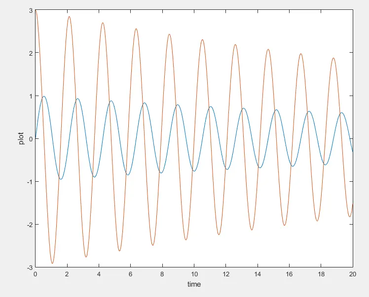
Fig 2 shows the resultant plot from the code

The youtube link for the video is : https://youtu.be/ef_iF3qbF_M

REFERENCES:

1. https://www.acs.psu.edu/drussell/Demos/Pendulum/Pendulum.html
2. https://en.wikipedia.org/wiki/Harmonic_oscillator