A Matlab code to perform curve fitting on a given data.

AIM : To write a code in Matlab to fit a linear and cubic polynomial for a given temperature vs Cp data.

THEORY : Curve fitting is a technique to fit a curve or mathematical relation to predict closest proximity to the real or experimental set of data. There is always an error as we are just approximating a function that relates to the data, and the main work hence is to predict this error and make it as minimum as possible.

The measure of how efficiently a curve fits the real set of data can be identified by obtaining these four quantities;

1. The Sum of Squared Errors(SSE)
2. R-square
3. Adjusted R-square
4. Root Mean Squared Error

FORMULAE USED :

We consider that x as independent variable and y as the dependent variable;

1. Linear polynomial can be shown as ax+b; where a and b are constant.
2. A cubic polynomial can be shown as a`x^3`+b`x^2`+cx+d where a,b,c and d are constants.
3. At any point i if f(x(i)) gives the value as given by the polynomial function used and y(i) gives the actual value as by the data then;

• SSE( Sum of Squared Errors) = `sum_(i=1)^n``|y(i)-f(x(i))|^2`
• The term R squared (`R^2`) = `(SSR)/(SSE)` where SSR = `sum_(i=1)^n (f(x(i))-mean)`where mean is the arithmetic mean of all the values of y resulting from data.
• Adjusted R-squared is the R-squared adjusted for the values of x that are insignificant. Radj = `1-[ ((1-R^2)(n-1))/(n-k-1)]` such that n = no. of values in data and k is the no. of insignificant independent variables.
• Root Mean Squared Error(RMSE) = `sqrt{sum_(i=1)^n (y(i)-f(x(i))^2]/n`= `sqrt( (SSE)/n)`

WORKFLOW :

PART 1 : Showing curve fitting by Linear and cubic polynomial

• The first part shows the curve fitting by using linear and cubic polynomials.
• "polyfit" and "polyval" commands are used to find the polynomial coefficients and the cp values predicted through polynomial functions respectively.
• step wise explanation is shown in the code itself.

CODE :

clear all
close all 
clc
cp_data= load('data'); % loads the data given and assigns it to variable cp_data
temperature=cp_data(:,1);% first column of the data are temperature values stored in variable temperature
cp=cp_data(:,2);% second column of the data are the cp values stored in variable called cp
 
% PART A : CUBIC POLYNOMIAL
% curve fitting assuming a cubic function
% ax^3 +bx^2+cx+d
 [co_efficient,S, mu]=polyfit(temperature,cp,3) % finds the coefficients of the polynomial best fit for the data
 predicted_cp = polyval(co_efficient,temperature,S,mu); % finding the values of cp through the polynomial obtained
 % Goodness parameters for cubic functions
 ssr3=0;
 sse3=0;
 n=0;
 for i=1:length(cp)
     b3=(cp(i)-predicted_cp(i))^2;
     sse3=sse3+b3; % finding Squared Sum of Errors
     m=mean(cp);
     c3=(predicted_cp(i)-m)^2;
     ssr3=ssr3+c3; % finding Sum of Square of Regressions
     
 end
     r_square3=ssr3/(sse3+ssr3); % finding the R-square parameter giving the goodness of curve
     rsme3=sqrt(sse3/length(cp)); % finding Root Mean Square Error value
     
 
 % Plotting for cubic function and comparing with actual data
 figure(1)
 plot(temperature,cp) % plots the curve for given data
 hold on
 plot(temperature,predicted_cp) %plots the predicted polynomial cp values with temperature
 xlabel('temperature')
 ylabel('cp')
 legend('actual values','predicted values')
 
 % PART B: LINEAR POLYNOMIAL
 % curve fitting assuming a linear function
 % ax+b=y
 co_efficient1=polyfit(temperature,cp,1);
 predicted_cp1=polyval(co_efficient1,temperature);
 % Predicting goodness of linear polynomial fitting
 sse1=0;
 ssr1=0;
 for j=1:length(cp);
     b= (cp(j)-predicted_cp1(j))^2;
     c= (predicted_cp1(j)-m)^2;
     sse1=sse1+b;
     ssr1=ssr1+c;
   
 end
  r_square1=ssr1/(sse1+ssr1);
 % Plotting for linear function and comparing with actual data
 figure(2)
 plot(temperature,cp)
 hold on
 plot(temperature,predicted_cp1)
 xlabel('temperature')
 ylabel('cp')
 legend('actual values','predicted value')
 

RESULTS :

1. The cubic polynomial is a better fit than linear polynomial for the given data as the R-squared value is better for cubic polynomial value than the linear polynomial.

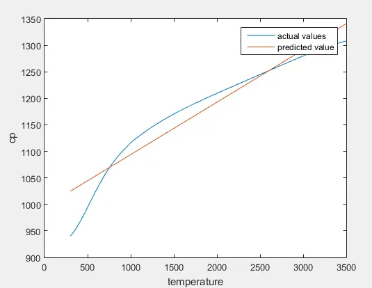
Fig 1 Plot showing visual distinction between actual data curve and linear fitted curve

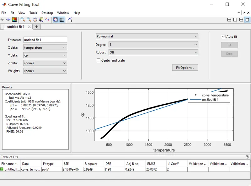
Fig 2 Plot by cftool a curve fitting tool in Matlab confirming Fig 1

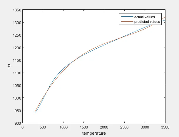
Fig 3 Plot showing visual difference between actual data curve and curve from cubic polynomial fit of data

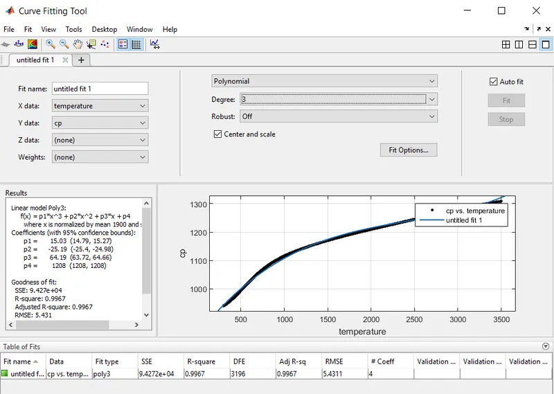
Fig 4 Plot from cftool a curve fitting tool in Matlab confirming Fig 3

PART 2 : Split-wise Method for curve fitting

1. In Split-wise method the data is divided into parts and the curve fitting is applied seperately for the parts.
2. Then we seperately apply curve fitting through polyfit and polyfit commands to different sets of data.
3. In this project the polynomial degree is kept 3 i.e. cubic polynomial.
4. Stepwise explanation is in code itself.

CODE :

% CURVE FITTING USING SPLIT-WISE METHOD
clc
clear all
close all
cp_data=load('data'); % loads data saved toa variable cp_data
cp=cp_data(:,2); % takes second column of loaded data(the cp values)
temp=cp_data(:,1);% takes first column of loaded data(the temperature values)
% SPLITTING DATA INTO DIFFERENT PARTS
temp1=temp(1:700); % fisrt set of  temperature data
temp2=temp(701:1400);% second set temperature data
temp3=temp(1401:2100); % third set of temperature data
temp4=temp(2101:2800); % fourth set of temperature data
temp5=temp(2801:3200); % fifth set of temperature data
cp1=cp(1:700); % first set of cp data
cp2=cp(701:1400);% second set of cp data
cp3=cp(1401:2100);% third set of cp data
cp4=cp(2101:2800);% fourth set of cp data
cp5=cp(2801:3200);% fifth set of cp data
% For first set of data
[c_eff1,S1,mu1]=polyfit(temp1,cp1,3); % finding coefficient by least square method 
predicted_cp1=polyval(c_eff1,temp1,S1,mu1);
sse1=0;
ssr1=0;
for i=1:length(temp1)
    a1=(cp1(i)-predicted_cp1(i))^2;
    sse1=sse1+a1;
    b1=(predicted_cp1(i)-mean(temp1))^2;
    ssr1=ssr1+b1;
end
r_squared1=ssr1/(ssr1+sse1);
rsme1=sqrt(sse1/length(temp1));
% For second set of data
[c_eff2,S2,mu2]=polyfit(temp2,cp2,3);
predicted_cp2=polyval(c_eff2,temp2,S2,mu2);
sse2=0;
ssr2=0;
for i=1:length(temp2)
    a2=(cp2(i)-predicted_cp2(i))^2;
    sse2=sse2+a2;
    b2=(predicted_cp2(i)-mean(temp2))^2;
    ssr2=sse2+b2;
end
r_squared2=ssr2/(ssr2+sse2);
rsme2=sqrt(sse2/length(temp2));
% For third set of data
[c_eff3,S3,mu3]=polyfit(temp3,cp3,3);
predicted_cp3=polyval(c_eff3,temp3,S3,mu3);
sse3=0;
ssr3=0;
for i=1:length(temp3)
    a3=(cp3(i)-predicted_cp3(i))^2;
    sse3=sse3+a3;
    b3=(predicted_cp3(i)-mean(temp3))^2;
    ssr3=sse3+b3;
end
r_squared3=ssr3/(ssr3+sse3);
rsme3=sqrt(sse3/length(temp3));
% For fourth set of data
[c_eff4,S4,mu4]=polyfit(temp4,cp4,3);
predicted_cp4=polyval(c_eff4,temp4,S4,mu4);
sse4=0;
ssr4=0;
for i=1:length(temp4)
    a4=(cp4(i)-predicted_cp4(i))^2;
    sse4=sse4+a4;
    b4=(predicted_cp4(i)-mean(temp4))^2;
    ssr4=sse4+b4;
end
r_squared4=ssr4/(ssr4+sse4);
rsme4=sqrt(sse4/length(temp4));
% For fifth and final set of data
[c_eff5,S5,mu5]=polyfit(temp5,cp5,3);
predicted_cp5=polyval(c_eff5,temp5,S5,mu5);
sse5=0;
ssr5=0;
for i=1:length(temp5)
    a5=(cp5(i)-predicted_cp5(i))^2;
    sse5=sse5+a5;
    b5=(predicted_cp5(i)-mean(temp5))^2;
    ssr5=sse5+b5;
end
r_squared5=ssr5/(ssr5+sse5);
rsme5=sqrt(sse5/length(temp5));
% OVERALL AVERAGE RESULT
r_square_avg= (r_squared1+r_squared2+r_squared3+r_squared4+r_squared5)/5;
rsme_avg=(rsme1+rsme2+rsme3+rsme4+rsme5)/5;
% PLOTTING
plot(temp,cp,'linewidth',6,'color','r') % plotting original data
hold on
plot(temp1,predicted_cp1,'linewidth',3,'color','b')% plotting polynomial prediction for first set
hold on
plot(temp2,predicted_cp2,'linewidth',3,'color','g')% plotting second set
hold on
plot(temp3,predicted_cp3,'linewidth',3,'color','y')% plotting third set
hold on
plot(temp4,predicted_cp4,'linewidth',3,'color','c')% plotting fourth set
hold on
plot(temp5,predicted_cp5,'linewidth',3,'color','m')% plotting fifth set
% legend command to mention the curves with their names in the plot
legend('original data','data1 fitting','data2 fitting','data3 fitting','data4 fitting','data5 fitting')
xlabel('temperature')
ylabel('cp')

RESULTS :

1. The split wise method has better results over non splitwise method of curve fitting. The R-squared value for cubic polynomial fit was around 0.9967 and for split-wise was 1.
2. For polynomial of higher order than 2 generally a warning is shown when centering and scaling is not done, hence for centering and scaling the syntax for polyfit command has to be changed a bit.

[p,s,mu]=polyfit(x,y,n) ; for this syntax matlab gives a vector mu such that mu(1) is average of x and mu(2) is

standard devation of x. Matlab centers x to zero and makes standard deviation 1 to increase numerical properties.

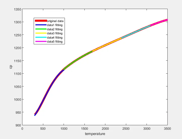
Fig 5 Plot obtained from split-wise curve fitting

Errors And Warnings faced

1. Few typos were encountered and were handled immediately.
2. Warning was faced when higher order polynomial were used, nd the command window gave warning that the polynomial was badly conditioned, Centering and scalling both manually in the code and by ticking option simply in cftool toolbox can avoid this.

Fig 6 Typing error committed in the code

Fig 7 Warning Matlab gives when centering and scaling is not performed for higher polynomials.

CONCLUSION :

1. Higher order polynomials give less error and fit better ,but increasing order to much causes large oscillations and complications. This phenomenon is called over-fitting.
2. Also Centering and scaling has to be done for higher order polynomials for better conditioning.
3. Split-wise method is a good option to make a better fit.

Based on these conclusions following questions can be asked:

Q1. How to make a curve fit perfectly?

Answer: For a perfect fit the value of R-square is 1 or approximately 1 and the curve overlaps the curve for actual data set. Split-wise technique is helpful for this.

Q2. How to get the best fit?

The best fit is that having the best R-squared value and low SSE value.

Q3. How to improve the cubic fit?

Centering and scaling to improve polynomial conditioning and split-wise technique can increase the cubic-fit.

REFERENCES :

1. https://skill-lync.com/student-projects/Curve-Fitting-and-criterion-to-choose-best-fit-41860
2. Help section of Matlab for polyfit centering and scaling