Week 4.1 - Genetic Algorithm

AIM:

To find the global maxima for the stalagmite function using genetic algorithm using Matlab.

OBJECTIVE:

To understand the concept og genetic algorithm

To understand the syntax for genetic algorithm in matlab.

THEORY:

GENETIC ALGORITHM:

A genetic algorithm is a search heuristic that is inspired by Charles Darwin's theory of natural evolution. This algorithm reflects the proess of natural selection where the fittest individuals are selected for reproduction in order to produce offspring of the next generation.

Natural selection:

The process of natrual selection starts with selection of fittest individuals from the population. They produce offspring which inherits the characteristics of the parents and will be added to the next generation. If parents have better fitness, their offspring will be better than parents and have a better chance at surviving. The process keeps on iterating and at the end, a generation with the fittest individual will be found

This nation can be applied for a search problem. We consider a set of solutions for a problem and select the set of best ones out of them.

Five phases are considered in a genetic algorithm.

1. Initial population. 2. Fitness function 3. Selection 4. Crossover 5. Mutuation

Initial population:

The process begins with a set of individuals which a set of individuals which is called a population. Each individual is a solution to the problem you want to solve.

Fitness function:

The fitness function determine how fit an individual is (ability of an individual to compete with other individuals). It gives a fitness score to each individual. The probability that an individual will be selected for reproduction is based on its fitness score.

Selection:

The idea os selection phase is to select the fittest individuals and let them pass their genes to the next generation. Two pairs of individuals (parents) selected based on their fitness scores, Individuals with high fitness have more chance to be selected for reproduction.

Crossover:

Crossover is the most significant phase in a genetic algorithm. For each pair of parents to be mated, a crossover point is chosen at random from within the genes.

Mutuation:

In certain new offspring formed, some of their genes can be subjected to a mutuation with a low random probability. This implies that some of the bits in the bit string can be flipped

Syntax for Genetic Algorithm in Matlab:

x = ga(func,nvars) x = ga(func,nvars,A,b) x = ga(func,nvars,A,b,Aeq,beq) x = ga(func,nvars,A,b,Aeq,beq,lb,ub) x = ga(func,nvars,A,b,Aeq,beq,lb,ub,nonlcon) x = ga(func,nvars,A,b,Aeq,beq,lb,ub,nonlcon,options) x = ga(func,nvars,A,b,[],[],lb,ub,nonlcon,Intcon) x = ga(func,nvars,A,b,[],[],lb,ub,nonlcon,Intcon,options) x = ga(problem) [x,fval] = ga(__) [x,fval,exitflag,output] = ga(__) [x,fval,exitflag,output,populaion,scores] = ga(__)

In this program,

[x,fval] = ga(func,nvars,A,b,Aeq,beq,lb,ub,nonlcon,Intcon,options)

x = optimum solutions

nvars = Number of variables, specified as a positive integer

A,b = Linear inequality constraints

Aeq,beq = Linear equality constraints

lb,ub = lower and upper bounds

nonlcon = use for nonlinear constrains

Intcon = to get solution in integer

options = optimization options

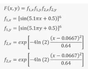
Formula for stalagmite function:

Matlab Program:

clear all
close all
clc

x = linspace(0,0.6,150);
y = linspace(0,0.6,150);
num_cases= 50;

% creating 2Dimensinal mesh
[xx, yy] = meshgrid(x,y);

% evaluating stalagmite function
for i = 1:length(xx)
    for j = 1:length(yy)
        input_vector(1) = xx(i,j);
        input_vector(2) = yy(i,j);
        f(i,j) = stalagmite(input_vector);
    end
end

% statistical behaviour

tic
for i = 1:num_cases
    [inputs,fopt1(i)] = ga(@stalagmite,2);
    xopt1(i) = inputs(1);
    yopt1(i) = inputs(2);
end
study_1_time = toc

% plotting
figure(1)
subplot(2,1,1)
hold on
surfc(x,y,f)
shading interp
plot3(xopt1,yopt1,fopt1,'marker','o','markersize',5,'markerfacecolor','r')
title('Unbounded inputs')
subplot(2,1,2)
plot(fopt1)
xlabel('Iteration')
ylabel('Function minimum')

% study2 - statistical behaviour with upper and lower bounds

tic
for i = 1:num_cases
    [inputs,fopt2(i)] = ga(@stalagmite,2,[],[],[],[],[0;0],[0.5;0.5]);
    xopt2(i) = inputs(1);
    yopt2(i) = inputs(2);
end
study_2_time = toc

% plotting
figure(2)
subplot(2,1,1)
hold on
surfc(x,y,f)
shading interp
plot3(xopt2,yopt2,fopt2,'marker','o','markersize',5,'markerfacecolor','r')
title('bounded inputs')
subplot(2,1,2)
plot(fopt2)
xlabel('Iteration')
ylabel('Function minimum')

% study3 increasing GA iterations

tic
options = optimoptions('ga');
options = optimoptions(options,'Populationsize',240);

for i = 1:num_cases
    [inputs,fopt3(i)] = ga(@stalagmite,2,[],[],[],[],[0;0],[1;1],[],[],options);
    xopt3(i) = inputs(1);
    yopt3(i) = inputs(2);
end
study_3_time = toc

figure(3)
subplot(2,1,1)
hold on
surfc(x,y,f)
shading interp
plot3(xopt3,yopt3,fopt3,'marker','o','markersize',5,'markerfacecolor','r')
title('bounded inputs eith modified population size')
subplot(2,1,2)
plot(fopt3)
xlabel('Iteration')
ylabel('Function minimum')

Starts the program with clear all, close all, clc which clear memory

Define the search space with x and y values and create 1D array for x and y using linspace command

Create 2D array based on 1D array using meshgrid command

To calculate stalagmite function for each value use for loop command and craete an array called input_vector(1) and input_vector(2) for each value of x an y and save these values in input_vector.

To calculate maxima, create a new function called stalagmite by using the above stalagmite formula and store the values in GA function.

function [F] = stalagmite(input_vector)

          x = input_vector(1);
          y = input_vector(2);

          f1_x = (sin(5.1*pi*x + 0.5)).^6;
          f1_y = (sin(5.1*pi*y + 0.5)).^6;    
          f2_x = exp(-4*log(2)*((x-0.0667).^2)/0.64);
          f2_y = exp(-4*log(2)*((y-0.0667).^2)/0.64);

          [F] = -(f1_x.*f1_y.*f2_x.*f2_y);

end

Then, this will call the function in for loop and passing the number of variables as input. So, the for loop will generate the data for plot.

Use three studies to get desired output(maxima)

Study1 - Statistical behaviour

Studt2 - Statistical behaviour with upper and lower bounds

Study3 - Increasing GA iterations

Study1 - Statistical behaviour:

After creating x and y variables (input variables), use num_case=50 means the code is going to run 50 times.

Use for loop to run the code 50 times, after that call the ga and use the new function @stalagmite, pass 2 varibles ( x and y) as inputs and store the output in fopt.

And then store the values of x and y in 'xopt' and 'yopt'.

To visualize the output use surface command (surfc) and use the shading command (shading interp) to get a smooth plot without the grid lines in new figure window(figure1)

Use tic-toc command to calculate the time taken for evaluation and also use subplot command for multiple plottinf in the same figure window

Studt2 - Statistical behaviour with upper and lower bounds:

In this study, use the same procedure of study 1 and setup the bound conditions for the variables x and y for above & below the 0 and 0.6.

Use genetic algorithm syntax and give x & y the upper limit and lower limit to 0 to 1.

Study3 - Increasing GA iterations:

In addition of specifying bounds increase initial population size. If population size is too small we cannot find the global maxima but ca find local maxima happens in study2.

By following the same procedure, increase the population size 240 and apply the constraint 'optimoptions' and save its values in the variable 'options' to allow the ga to predict the optimum solution for 240 poulation size.

RESULTS:

Study1 - Statistical behaviour

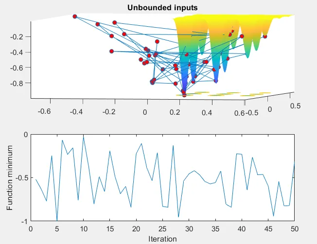
Here on plotting the stalagmite function and aslo plotting the minimum value that ga predicts, which is all over the place on graph, it happens due to random sample during each iteration the value changes. In the command window, we can observe the time taken for iteration is 5.4476sec.

Studt2 - Statistical behaviour with upper and lower bounds

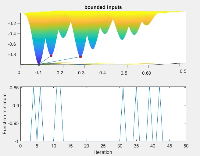
From the graph, the function predict minimum point is between 3 peaks. It is accurate but not clear. In the command window, we can observe the time taken for iteration is 6.8021sec higher than study1.

Study3 - Increasing GA iterations

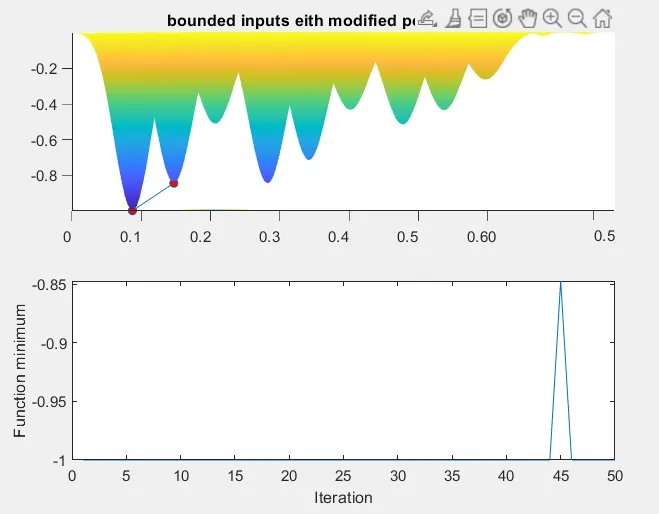
From the graph, maxima only lies around peak1 and its around the value 0.85 that ga predicts. In this study its giving the optimum value, on increasing the number of itertion and applying constraints .We can observe the time taken for iteration is 22.0661sec which is 4 times higher than study1.

Error Faced:

I put 'fop3t' instead of 'fopt3'.